The Slide Rule
The slide rule is an analogue calculating device that first appeared during the first half of the seventeenth century CE. Its invention is usually attributed to the English mathematician and Anglican clergyman William Oughtred (1574-1660). Like many inventions, his device was based on the work of a number of other individuals, predominant among whom were the Scottish mathematician John Napier (1550-1617) and the English mathematician Edmund Gunter (1581-1626).
Napier's contribution was the discovery of logarithms. Napier spent over two decades working on the theory of logarithms, and eventually published his findings in his 1614 work Mirifici Logarithmorum Canonis Descriptio (A Description of the Wonderful Law of Logarithms), just three years before his death at the age of sixty-seven.
The logarithm of a number x is the exponent (i.e. power) y by which another number (known as the base, b) must be raised in order to produce x. The base used can vary, depending on the area of application. In computer science, a base of two is often used, while in pure mathematics and many scientific applications a base known as e is used. In engineering and electronics, base ten is frequently used, and is obviously well suited for use with a decimal number system.
Napier found that the logarithm of the product of two numbers is equal to the sum of the logarithms of the individual numbers. The process of multiplying two large numbers together can thus be greatly simplified by adding together the logarithms of the two numbers and taking the antilogarithm of the result. The antilogarithm is the inverse function of the logarithm – it returns the number for which another number is the logarithm to a given base. In other words, if x is the logarithm of y, then y is the antilogarithm of x.
The same principle can be applied to finding the quotient of two numbers (i.e. dividing one number by another). The difference is that in order to divide one number by another, we must find the difference of the logarithms of the two numbers and take the antilogarithm of the result. The principle is embodied in the first and second laws of logarithms, which can be stated as follows:
logb (m × n) = logb (m) + logb(n)
logb (m ÷ n) = logb (m) – logb (n)
Although the use of logarithms to find the product of two numbers does reduce a multiplication problem to one of simple addition, it also relies on the availability (and accuracy) of a set of logarithmic tables. In order to calculate the product of two numbers, we must first extract the logarithm of each number from the tables. Once we have added the two logarithms together, we then have to use the tables once more to look up the antilogarithm of the result.
Napier's logarithms were natural logarithms, i.e. logarithms to base e (c. 2.7183). Natural logarithms are of great interest to mathematicians, especially those involved in the pursuit of pure mathematics, but they are not so useful for engineers and scientists, who tend to work with decimal values (i.e. numbers to base ten).
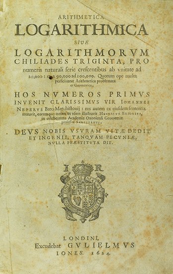
In 1617, the English mathematician Henry Briggs (1561-1630), who had been influential in encouraging the adoption of Napier's ideas, suggested the use of a decimal base instead of e. With Napier's agreement, he undertook the creation of a set of logarithmic tables to base ten, and in 1624 published his work Arithmetica Logarithmica, which contained the logarithms to base ten of thirty thousand natural numbers (1 – 20,000 and 90,001 – 100,000) to fourteen decimal places.
The scientific community were quick to adopt the use of logarithms in order to reduce the time and effort required for computation, especially in the field of astronomy, where it was often necessary to carry out long and tedious calculations involving very large numbers. The contributions of Napier and Briggs led to the development in 1620 of a precursor to the slide rule – the Gunter scale.
The Gunter scale was a logarithmic scale invented by Edmund Gunter as a navigational aid for mariners. The original scale consisted of a single length of metal or wood with markings etched into it at intervals, numbered from 1 to 10. The intervals were spaced in proportion to the logarithm of the number each represented. The distance between 1 and 2 is equal to 0.3 units; the distance between 1 and 4 is 0.6 units; that between 8 and 1 is 0.9 units; and so on. Navigators could make calculations involving multiplication and division using a "Gunter" (as it became known) and a set of dividers, or calipers.
In (circa) 1622 William Oughtred invented the earliest form of the slide rule, which was circular. The device utilises an inner ring, and an outer ring that can slide around each other. Each ring has an identical logarithmic scale engraved on it. The illustration below shows an instrument made by the Scottish instrument maker Robert Davenport based on a description in Oughtred's original Latin manuscript Circles of Proportion and the Horizontal Instrument, which he wrote in (circa) 1632, and which was later translated into English and eventually published by Oughtred's student William Forster in 1660.
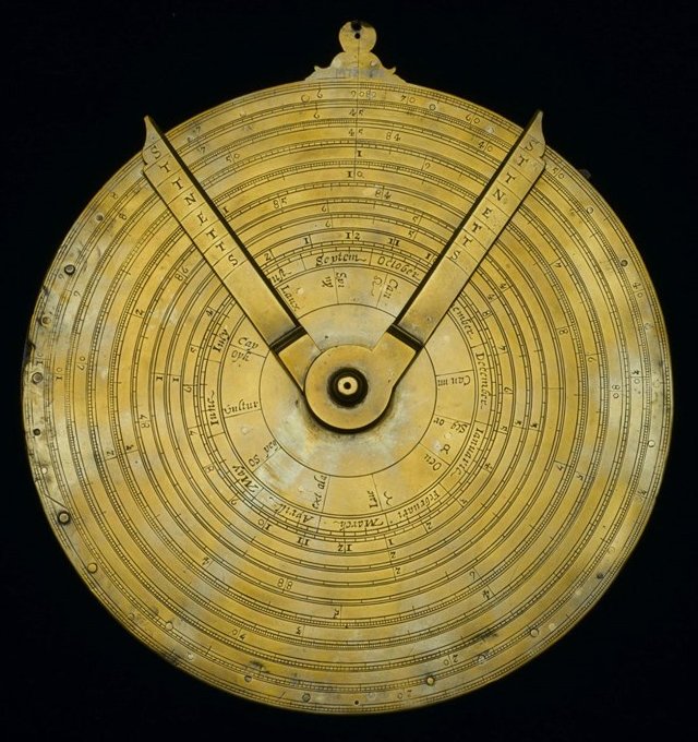
Even though Oughtred's design was for a circular instrument, it was based on the principle of using two identical Gunter scales in tandem, by sliding one past the other in order to carry out calculations. The illustration below shows how we might use such a pairing to calculate the product of two and four (2 × 4). We start by sliding the upper scale to the right until the interval marked "1" on the upper scale lines up with the interval marked "2" on the lower scale. We then read off the value on the lower scale that is aligned with the interval marked "4" on the upper scale, which gives us the answer eight (8).
Using two Gunter scales to find 2 × 4
In fact, as you can see from the illustration, once we have aligned the "1" on the upper scale upper scale with the "2" on the lower scale, we can read off the value of two multiplied by any value up to and including five (5) by finding that value on the upper scale and reading off the corresponding value on the lower scale. Which raises another question: how do we multiply two by a value that is greater than five? Suppose, for example, we want to multiply two by seven (2 × 7)?
When the "1" on the upper scale is aligned with the "2" on the lower scale, the "7" on the upper scale is not aligned with anything at all. We get around the problem by aligning the "10" on the upper scale (i.e. the right-hand index of the upper scale) with the "2" on the lower scale instead. This means that any value we read off on the lower scale will be one tenth of the value we are looking for. As you can see, the "7" on the upper scale corresponds to a value of 1.4 on the lower scale. All we need to do to get the correct result is move the decimal point one place to the right.
Using two Gunter scales to find 2 × 7
Finding the quotient of two numbers (i.e. dividing one number by another) is also relatively straightforward. Suppose, for example, we want to divide five by two (5 ÷ 2). We move the "2" on the upper scale so that it lines up with the "5" on the lower scale. We then read off the result on the lower scale by finding the value that corresponds to the "1" on the upper scale, which in this case is 2.5.
Using two Gunter scales to find 5 ÷ 2
We can manipulate the scales in various ways to find the sum and quotient of any two numbers, regardless of how big or how small they are. Once we have a result, we just need to determine where the decimal point goes. This is often a matter of mentally calculating an approximate result so that we know how far to the left or the right we need to shift the decimal point in the value read from the slide rule in order to get the correct answer.
The slide rule gradually evolved from a simple pairing of Gunter scales into a somewhat more sophisticated instrument. In 1654, it began to look more like the slide rule we are familiar with today, when the English instrument maker and inventor Robert Bissaker (1620-1685) made a slide rule consisting of three parallel rules. The two outer rules were fixed with respect to one another. Between them was an inner sliding rule.
In 1775, the English mathematician John Robertson (1712-1776) produced the first slide rule to have a runner (or cursor). Robertson's cursor took the form of a simple sliding brass rectangle mounted on top of the scales. The cursor later evolved into a sliding window made of glass or plastic, with a line etched into it that ran perpendicular to the scales. The cursor serves as both a placeholder and as a method of transferring settings from one scale to another.
n 1851, French army officer Amédée Mannheim (1831-1906) created what was essentially to become the standard version of the slide rule, and one that has endured with only minor modifications up until the present day. Mannheim's instrument was designed as a general-purpose slide rule for making all kinds of scientific and engineering calculations. It had all of the characteristics so far described, including two fixed parallel rules, one sliding rule, and a cursor (Mannheim's slide rule had a much thinner cursor than Robertson's, allowing more of the scales to be seen).
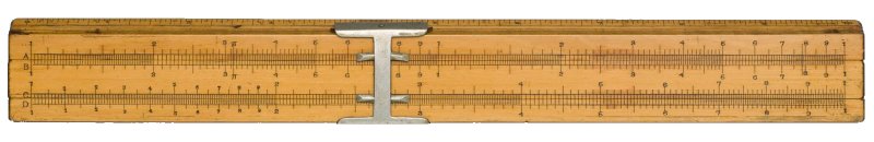
The illustration above shows a French-made Mannheim slide rule dating from some time in the late nineteenth century CE. The main innovation introduced by Mannheim was the arrangement of the scales (see below). Each of the fixed parallel rules had a scale on its inside edge. The sliding rule, which lay between them, had a scale on each of its outer edges, with each scale corresponding to the scale on the fixed rule to which it was adjacent.
The two outermost scales are designated as A and D, while the scales on the sliding rule are designated B and C. Scales A and B are double decade scales, and are used for finding squares and square roots. Scales C and D are single decade scales, and are used for multiplication and division (single decade scales range from 1 to 10 over the length of the slide rule, whereas double decade scales range from 1 to 100).
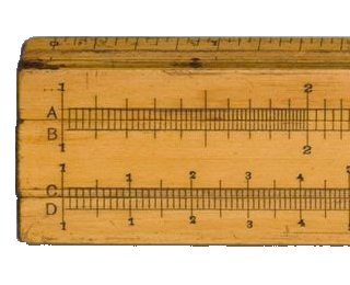
Enlarged view of Mannheim slide rule, showing the A, B, C and D scales
From 1851 until the latter half of the twentieth century, many variants of Mannheim's slide rule emerged, but the underlying format remained the same. Additional scales were added to allow the calculation of cubes and cube roots, logarithms and exponentials, trigonometric functions, reciprocals, and various other functions. Slide rules became available that had additional scales on their reverse side. These instruments became known as duplex slide rules (slide rules with scales on one side only are referred to as simplex slide rules).
Towards the end of the eighteenth century, the slide rule became an essential tool for engineers and scientists, and would remain so until the late 1970s. It enabled calculations to be made quickly, and with a precision of between two and three significant digits, depending on the skill of the user and the ease with which the scales could be read (this could vary somewhat, depending on the quality of the instrument – good quality slide rules were quite expensive).
The slide rule was essentially a versatile and highly portable analogue computing device that did not require batteries or a power source. On the down side, its accuracy was limited in comparison with the digital electronic calculators that would eventually replace it. Learning to use a slide rule could also be a daunting proposition, because it required at least a basic understanding of the mathematical principles involved.
The first hand-held pocket calculator was Hewlett Packard's HP-35, which first appeared on the market in 1972 and retailed for just under four hundred dollars. Although still beyond the reach of most students at that time, the HP-35 signalled the imminent demise of the slide rule. It was far more accurate, much easier to use, and just as portable. Prices fell rapidly as more and more manufacturers brought their products onto the market, and within a few short years the slide rule had become virtually obsolete.