Functions and Graphs
Overview
Although there is evidence that the concept of a function was emerging as early as the fourteenth century CE, it was German philosopher and mathematician Gottfried Leibniz who, towards the end of the seventeenth century CE, first coined the term function. Leibniz used the term to describe the algebraic relationship between the x and y coordinates of any point on a geometrically derived curve such as a tangent or chord, but the idea was later generalised to include any algebraic relationship in which the value of an output y (known as the dependent variable) is functionally dependent on the value of an associated input x (known as the independent variable). The input of the function is alternatively referred to as its argument, while the output of the function may also be referred to as its value. A function produces one (and only one) output for any given input. Although for the purposes of this discussion we will assume that the inputs and outputs of a function are real numbers (essentially, any number that is not an imaginary number), they may take other forms. Here is an example of a function:
ƒ(x) = 3x
This is the standard notation for defining a function named ƒ. The action of this function is to produce an output for any given input value (x). The output is equal to x multiplied by three. Thus, we could apply the function as defined to a specific input value as follows:
ƒ(5) = 15
It is common when writing algebraic expressions to call the input of a function x, and the output of the function y. If we were to describe the action of the function defined above using an algebraic equation, we could say:
y = 3x
Writing an equation is only one of the ways in which we can describe a function, however. There are several other ways of expressing the action of a function. The first of these is to make a table consisting of a range of possible input values together with their corresponding output values. Note that a set of ordered pairs in which each pair consists of an input value and an output value is known as a relation. If we create a table of inputs and outputs for the function ƒ(x) = 3x, we could get something like the following:
| x | -5 | -4 | -3 | -2 | -1 | 0 | 1 | 2 | 3 | 4 | 5 |
| 3x | -15 | -12 | -9 | -6 | -3 | 0 | 3 | 6 | 9 | 12 | 15 |
We can also view the function as a graph by plotting values of x and y on graph paper and joining the points together using a straight line or a curve (depending on whether the function is linear or non-linear). Note that most spreadsheet programs currently available will also produce a graph based on a given set of input and output values. In fact, you can simply enter the function into the spreadsheet as a formula and let the spreadsheet calculate the output values for a range of inputs. The following illustration is a screenshot of a graph produced using Microsoft Excel in this manner, using the input (x) values from the above table:
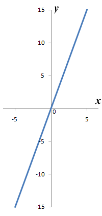
The graph of the linear function ƒ(x) = 3x
If a function's output can be expressed using an algebraic equation, it is said to be computable. The word computable here means that we can calculate the output for any given input. In most cases, the calculation can either be carried out using a pencil and paper, or may be implemented as a computer algorithm. The set of all possible values that can be used as the inputs for a particular function is called the function's domain. The set of all possible values that can be produced as outputs for a function is called the co-domain. If the function can accept real-valued inputs, both the domain and the co domain could include all of the real numbers, depending on the action defined for the function. This is certainly the case for the function ƒ(x) = 3x. We could thus theoretically extend the graph for this function for an infinite distance in either direction. Note however that if the domain (i.e. the set of possible input values) for the function ƒ(x) = 3x were restricted to the set of integers, the co-domain would also be restricted to the set of integers, and the set of possible output values (sometimes referred to as the function's range or image) would be restricted to the set of integers that are also multiples of three, plus zero.
A function is sometimes described in terms of its relationship with another function. The most frequently occurring example of this is the inverse function of a given function. We can say, for example, that the inverse of the power function ƒ(x) = 10 x is the logarithmic function log10 x. The inverse of a function reverses the action of the original function. For example, if we apply the power function ƒ(x) = 10 x to a value for x of two, we get the following:
ƒ(2) = 10 2 = 100
Theoretically therefore, if we apply the logarithmic function log10 x to this output, it should reverse the action of the power function and restore the value of x to its original value (two). Here is the result of applying the inverse function:
ƒ(100) = log10 100 = 2
Not all functions can have an inverse function. A function that can have an inverse function is said to be invertible. A familiar example of an invertible function is the function that converts a temperature in degrees Celsius (C) to the temperature in degrees Fahrenheit (F):
| F = ƒ(C) = | 9 | C + 32 |
| 5 |
The inverse function of a function ƒ is frequently designated as function ƒ -1. The inverse of the above function (i.e. the function that would convert the temperature from degrees Fahrenheit back to the temperature in degrees Centigrade) could thus be written as follows:
| C = ƒ-1(F) = | 5 | (F - 32) |
| 9 |
Finding the domain of a function
As previously stated, the domain of a function is the set of all possible input values. The domain will include any input value that results in a real number output. If there are no restrictions on the possible real-valued inputs for a function, the domain consists of the set of all real numbers. For some functions, this will not be the case. If the function produces a quotient (i.e. the result of a division operation) in which the input is the denominator, then zero cannot be included in the function's domain. A zero-valued denominator would result in division by zero, and the output would therefore be undefined. Similarly, if the function produced an output that involved a square root, the input value would need to be chosen in order to avoid an attempt to calculate the square root of a negative number, since a negative number cannot have a square root. Consider the following functions:
ƒ(x) = 3x 2 - 4x + 2
ƒ(x) = √(x + 16)
In the first example above, it can be shown that we can input any real-valued number for x and get a real number as the output, so the domain of the function ƒ(x) = 3x 2 - 4x + 2 is all of the real numbers. In the second example, we have an output that is the square root of x plus sixteen (x + 16), so x must be equal to or greater than minus sixteen (-16). Only values of x that are greater than or equal to minus sixteen will give a radicand that is guaranteed to have a value of zero or greater (the radicand is the term whose root is being taken). The domain for the function ƒ(x) = √(x + 16) is therefore all of the real numbers with a value of minus sixteen or above.
Linear functions
Linear functions are so called because their graph is invariably a straight line (as opposed to a curve). The things that are of interest to us when we are looking at the graph of a linear function are the slope of the line, and the points at which the line crosses the x and y axes on the graph. Note that constant functions are a special case of the linear function in which the line is horizontal and never crosses the x-axis - see below. Note also that the line cannot be vertical, since this would imply that x was a constant. If this were the case, we would not be dealing with a function, since y would not be dependent upon x. The points at which the line intercepts the x- and y-axes, and hence its slope, are determined by the equation that describes the function. The general form of a linear function can be expressed as follows:
y = ƒ(x) = mx + c
Here, x and y are variables and m and c are constant values. It can be shown that m is the slope (or gradient) of the line and c is the value of x at which the line intercepts the y-axis. An equation written in this form is said to be in slope-intercept form. For any given linear equation, we can find values for y by plugging various values of x into the equation. If we find a sufficient number of values for y (two would be the minimum), we can draw the graph. We could also carry out an analysis of a straight line graph to derive the equation for the function relatively easily. We can find the value of c simply by finding the y intercept. The value of m is the slope of the line, and can be found by taking the x and y coordinates of two suitable points on the line and applying the following formula:
| m = | Δy | = | y2 - y1 |
| Δx | x2 - x1 |
Consider the following graph:
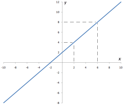
The graph of a linear function
We can see from the graph that the line intercepts the y axis where y equals two (y = 2), so the value of the constant c is two. Taking values for x1 and x2 of two and six (2 and 6), we can see that the corresponding values for y1 and y2 are four and eight (4 and 8). We can now substitute these values into the formula for the slope of the line as follows:
| m = | Δy | = | y2 - y1 | = | 8 - 4 | = | 4 | = 1 |
| Δx | x2 - x1 | 6 - 2 | 4 |
The value of m (i.e. the slope of the line) is therefore one (1), and we can write the equation for the function that describes the graph as follows:
y = ƒ(x) = x + 2
Note that if the slope of the line is negative (i.e. the line slopes downwards from left to right), then the value of m will also be negative. There are some further points to note. First, if two linear functions produce graphs with the same slope but different y-intercepts, they are parallel (if both the slope and the y-intercepts are equal, then the functions are identical). Second, if the product of the slopes of two lines equals minus one (-1), then the graphs will be perpendicular (at right angles) to each other. Finally, for a linear function, if the slope and one point on the line are known, or alternatively if any two points on the line are known, the graph of the function can be drawn and its equation identified.
Be aware also that by no means all linear functions have a domain that is the set of all real numbers. Some functions produce a discontinuity. To illustrate this, consider the following function:
| y = ƒ(x) = | 2x 2 - 5x + 3 |
| x - 1 |
You should be able to see that for this function, when x is equal to one, the value of y will be undefined because x minus one (x - 1) in the denominator will result in division by zero. No other real number values of x will cause a problem, so there is essentially a gap in the graph consisting of a single point on what is otherwise a continuum. Here is the graph for the function (note that the discontinuity is indicated using a small circle):
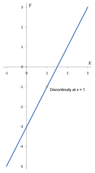
The graph of a discontinuous linear function y = ƒ(x) = (2x 2 - 5x + 3) / (x - 1)
If a linear equation has two (or more) unknown values, it is going to be virtually impossible to solve without more information. If on the other hand we have two different equations, both of which relate to the same unknown values, then we can solve both of the equations at the same time (i.e. simultaneously). Solving these "simultaneous equations" algebraically will not be dealt with here. What is of interest to us at the moment is the fact that, for linear equations involving two variables (x and y), we can draw a straight line graph based on what we do know. If we have two equations that refer to the same unknown values, we can draw two graphs. Although this sounds like stating the obvious, the point is that by drawing the graph of both equations on the same set of axes, we can immediately see where the lines intercept each other (assuming that they do, of course). The point at which they intercept will have the x and y coordinate values that satisfy both equations. Let's assume that we have been given the following equations:
2x + y = 7
3x - y = 8
We can draw the graphs for both equations on the same set of axes as follows:
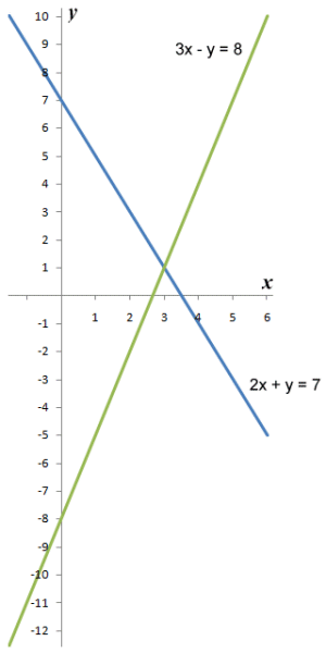
The graphs of linear equations 2x + y = 7 and 3x - y = 8
From the graphs, we can see that the intercept occurs at coordinates x = 3, y = 1. We can check that the values are correct by plugging them into both equations to make sure that we get the stated result in both cases. If the equations are the same, we will get the same graph in both cases. This effectively means that all points on the line are solutions. If the lines do not meet, they must (by definition) be parallel, and there is therefore no solution.
Constant functions
A constant function is one in which the output value never changes. We can write a generic constant function ƒ(x) = c, in which c is some (unspecified) constant value. The output of the constant function ƒ(x) = c never changes, regardless of the value taken by x. A real world example of a constant function would be the function that relates the quotient of force (F) and acceleration (a) to the mass (m) of a body (note that the mass m of a body is a constant, unlike its weight, which depends on the force acting on the body due to gravity):
ƒ(F/a) = m
The constant function is the simplest kind of function to describe algebraically because its output does not vary. For the same reason the graph of a constant function is also very simple. The graph of a function is a line or curve connecting a set of x and y coordinates representing the input values and corresponding output values of the function. Since the output values (represented by the y coordinates) will always be the same regardless of the value of the input values (represented by the x coordinates), then the graph of the constant function ƒ(x) = c is the horizontal line that passes through the y axis at the coordinates 0, c. Here is the graph for the constant function ƒ(x) = 3:
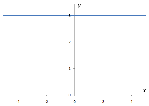
The graph of constant function ƒ(x) = 3
Quadratic functions
Quadratic equations are used to solve all kinds of problems in science, engineering, and many other fields. A quadratic function is a polynomial function that takes the form ƒ(x) = ax 2 + bx + c, in which a, b and c are constants, and a cannot equal zero. The graph of a quadratic function is a parabola, with an axis of symmetry that is parallel to the y axis (see below). The term quadratic refers to the fact that the highest exponent present in the expression that describes the function is two (2). This means that the function is a second order polynomial. If the output of the function is set to zero, the resulting equation is a quadratic equation (i.e. it takes the form y = ƒ(x) = ax 2 + bx + c = 0). The solution of a quadratic equation is the value (or values) of x for which this is true (i.e. y equals zero). Looking at the graph of a quadratic function, it should become evident that for any given quadratic equation there are three possible outcomes:
- the graph does not intercept the x-axis, and there is no solution
- the graph intercepts the x-axis at a single point, and there is one solution
- the graph intercepts the x-axis at two points, and there are two solutions
In most cases, we would expect to see the graph intercept the line at two points. The x coordinates corresponding to these points are called the roots of the equation. We can therefore find the solution to a quadratic equation by drawing the graph of the function and finding the points at which the graph intercepts the x-axis. Here is the graph for the function y = ƒ(x) = x 2 - 4x - 5:
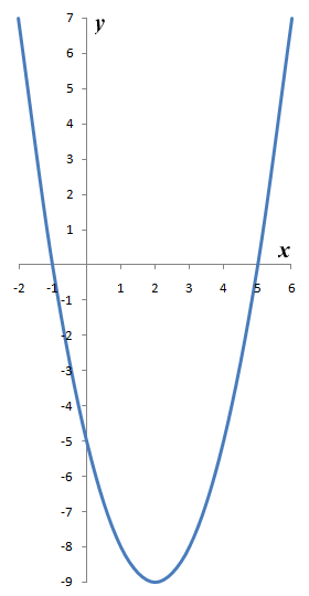
The graph of y = ƒ(x) = x 2 - 4x - 5
We can see from the illustration that the graph intercepts the x-axis at two points: x equals minus one (x = -1) and x equals five (x = 5). There are therefore two solutions (minus one, and five) for the quadratic equation x 2 - 4x - 5 = 0. You can see the characteristic shape of the graph here. The bottom of the graph (or the top, it the parabola is inverted) is called the apex or turning point. If the apex lies on the x axis, there is only a single solution. Depending on the values of a, b and c in the quadratic function, the precise shape and position of the parabola will vary. If the value of a is negative, for example, the parabola will be inverted (upside down, with the apex at the top rather than the bottom).
Cubic functions
Like quadratic equations, cubic equations are used to solve problems in science, and engineering. A cubic function is a polynomial function that takes the form ƒ(x) = ax 3 + bx 2 + cx + d, in which a, b, c and d are (usually) real numbers, and a cannot equal zero. The graph of a cubic function is a curve, as shown below. The term cubic refers to the fact that the highest exponent present in the expression that describes the function is three (3). This means that the function is a third order polynomial. If the output of the function is set to zero, the resulting equation is a cubic equation (i.e. it takes the form y = ƒ(x) = ax 3 + bx 2 + cx + d = 0). The solutions of a cubic equation are the values of x for which this is true (i.e. y equals zero). The graph of a cubic function intercepts the x axis at three points, and a cubic equation therefore has three roots. We can find the solution to a cubic equation by drawing the graph of the function and finding the points at which the graph intercepts the x axis. Here is the graph for the function y = ƒ(x) = 2x 3 - 3x 2 - 3x + 2:
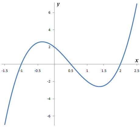
The graph of y = ƒ(x) = 2x3 - 3x 2 - 3x + 2
We can see from the illustration that the graph intercepts the x axis at three points. There are therefore three solutions for the cubic equation 2x 3 - 3x 2 - 3x + 2 = 0. The solutions for the graph shown here are: x = -1, x = 0.5 and x = 2. The points on the graph where the curve undergoes a sharp change in direction are called the critical points. The graph shown above has two critical points.
