Angle Modulation
Overview
Modulation is the process of varying the properties of a periodic waveform in order to represent analogue or digital information. The periodic waveform used is called a carrier, and usually has a sinusoidal waveform. The property that is varied by the modulation process depends on the kind of modulation scheme being used. It could be the amplitude, frequency, or phase of the carrier wave, or even some combination thereof.
The underlying reason for wanting to modulate an information-carrying signal onto a carrier wave is that the signal is unsuitable for the transmission medium over which we want to send it. An example that most people will be familiar with is broadcast radio, which typically broadcasts music, news, weather forecasts and so on. The frequencies we actually hear when we listen to a radio broadcast belong to the audio spectrum, which ranges from about 20 Hz at the lower end up to around to 20 kHz at the extreme upper limit of hearing.
Sending audio-frequency signals over a wired transmission line is not a problem, although the public switched telephone system limits the frequencies used to between 300 and 3,400 hertz, giving a total bandwidth of 3,100 hertz. This is perfectly adequate for purely voice transmission, since the higher frequencies in the human voice (i.e. those above 3,400 hertz) are not really needed for recognisable speech reproduction. The use of a limited bandwidth also makes the telephone system much easier to implement and maintain from an engineering perspective.
Sending audio signals wirelessly using radio frequencies is not so easy. The audio spectrum spans the extremely low frequency (ELF), super low frequency (SLF), ultra low frequency (ULF), and very low frequency (VLF) bands, which cover the range from 3 Hz up to 30 kHz. Apart from the fact that most of these frequencies are used for highly specialised military applications, there is another more serious problem.
It turns out that the size of the antenna needed to transmit radio waves is inversely proportional to the frequency of those radio waves; the antennae needed to transmit at these frequencies can vary in length from a few kilometres up to several tens of kilometres! In order to broadcast audio signals in a cost-effective and efficient manner, we need to use higher frequencies. In order to get a high frequency signal to "carry" a low frequency signal, we have to use some form of modulation.
In this section, we have already looked at amplitude modulation (AM), which varies the amplitude of a high-frequency carrier in proportion to the instantaneous amplitude of a low-frequency information-carrying signal - usually an audio frequency signal. In this article, we will be looking at angle modulation, which varies the phase angle of the carrier in some way according to the instantaneous amplitude of the information signal.
The two primary forms of angle modulation are phase-modulation (PM), which uses the information-carrying signal to vary the instantaneous phase angle of the carrier, and frequency modulation (FM), which uses the information signal to vary the instantaneous frequency of the carrier. Most angle modulation schemes, whether they employ phase modulation or frequency modulation techniques, use the very high frequency (VHF) band, which occupies frequencies from 30 MHz up to 300 MHz, to transmit. The VHF carrier is modulated by a continuously varying analogue signal - in most cases an audio signal - that directly represents the information we want to transmit.
For two-way voice communications, where audio quality at the receiver is not a critical factor, either phase modulation or narrow-band frequency modulation may be used. In terms of purely analogue communication, the biggest application of phase modulation is in mobile radio services, although it is also used in many kinds of digital modulation scheme, which we will be looking at in some depth elsewhere. For commercial radio broadcasting, where audio quality is important, wideband FM has now largely replaced AM as the method of choice (we'll be looking at the differences between narrow-band and wideband in due course).
Frequency modulation has a better signal-to-noise ratio than phase modulation, and is thus less susceptible to noise, although both forms of angle modulation are superior to amplitude modulation in this respect. The amplitude of an angle-modulated signal, and hence the average transmitted power, is maintained at a constant level; all of the information carried by the angle-modulated signal is encoded as variations in either phase or frequency, and the effect of additive noise is far less significant than it is for amplitude modulation schemes.
Amplitude modulation is a linear modulation scheme because the bandwidth of each sideband is equal to that of the modulating signal. The two sidebands are mirror images of each other, each carrying the same information as the modulating signal itself. Angle modulation schemes are said to be non-linear, because the effective bandwidth does not depend on the bandwidth of the modulating signal, but on the modulation depth, as we shall see. Furthermore, most of the transmitted signal power resides in the sidebands rather than in the carrier itself, making angle modulation more power-efficient than amplitude modulation.
The trade-offs are that angle modulation schemes require more transmission bandwidth than amplitude modulation, and both transmitter and receiver circuitry are considerably more complex.
Frequency vs. phase
Both frequency and phase modulation vary the phase angle of a sinusoidal carrier in some way, based on the instantaneous amplitude of the modulating baseband signal, whilst maintaining the carrier signal at a constant amplitude. These complementary forms of modulation are thus very closely related.
For an RF carrier modulated by a sinusoidal (single-frequency) audio signal, and assuming that one of the two forms of angle modulation (FM or PM) has been used, then a visual inspection of the waveform is not particularly informative because it will have the same shape in either case. The resulting FM and PM waveforms are identical except for their relationship to the modulating signal in the time domain. The diagram below illustrates this relationship. The significance of the numbered points on the diagram depends on which form of angle modulation is being used.
A baseband signal is used to vary the phase or frequency of a high-frequency carrier
For a frequency-modulated signal, the maximum positive deviation from the centre frequency occurs when the modulating signal is at its maximum value (point 1), while the maximum negative deviation occurs when the modulating signal is at its minimum value (point 3). When the amplitude of the modulating signal is zero (points 2 and 4), the frequency deviation is also zero.
For a phase-modulated signal, the maximum negative deviation from the centre frequency occurs when the amplitude of the modulating signal is zero, and changing from positive to negative (point 2). The maximum positive deviation occurs when the amplitude of the modulating signal is zero, and the amplitude is changing from negative to positive (point 4). These zero-crossing points are where the rate of change of the modulating signal's amplitude is greatest. The frequency deviation is zero when the modulating signal is at its maximum positive or negative values (points 1 and 3).
In both forms of angle modulation, both the instantaneous phase angle and frequency of the carrier are dependent on the instantaneous amplitude of the modulating signal. Phase modulation changes the phase angle of the carrier in accordance with the amplitude of the modulating signal, leading to a corresponding change in carrier frequency, whereas frequency modulation changes the frequency of the carrier, resulting in a change in the carrier's phase angle. In neither case does the modulated waveform bear any resemblance to the modulating waveform.
In order to fully understand angle modulation, and the relationship between phase modulation and frequency modulation, we need to undertake a somewhat more mathematical analysis. We'll start with the basics. If we take the instantaneous phase angle in radians at time t of an angle modulated carrier to be φ (t), then the general form of the angle modulated wave s(t) can be expressed as:
s(t) = Ac cos [φ (t)]
where Ac is the carrier amplitude.
Let's assume that the phase angle increases monotonically with time. A monotonic function is one in which the dependent variable (in this case the phase angle) - either stays the same, only increases in value, or only decreases in value with respect to the independent variable (which in this case is time).
Here, the value of the phase angle is increasing with respect to time, although not necessarily at a constant rate. The phase angle of the modulated wave must undergo a change of 2π radians in in order to complete one oscillation. If the phase angle increases by Δφ over time interval Δt, we can express the average frequency of the modulated wave as follows:
| favg = | Δφ(t) |
| 2πΔt |
If we allow time interval Δt to approach zero, we can derive the following expressions for the instantaneous frequency f(t) of the angle modulated signal s(t):
| f(t) = | lim | Δφ(t) | |
| Δt→0 | 2πΔt |
| f(t) = | 1 | dφ(t) | |
| 2π | dt |
It follows from the above that the instantaneous angular frequency, ω(t), of the angle modulated signal in radians per second could be written as:
| ω(t) = | dφ(t) |
| dt |
This demonstrates an important point with respect to the relationship between frequency and phase, which is that the instantaneous angular frequency of a signal is the derivative of its instantaneous phase angle with respect to time. It follows that, by definition, the instantaneous phase angle is the integral of its instantaneous angular frequency with respect to time:
| φ(t) = φ(0) + | ∫ | t | ω(t) dt |
| 0 |
where φ(0) is the phase angle at time t = 0.
Because of the way in which phase and frequency are related, it is possible to produce a frequency-modulated signal using a phase modulator by first integrating the information signal, and then sending the output of the integrator circuit to the phase modulator. Conversely, it is also possible to produce a phase-modulated signal using a frequency modulator by first differentiating the message signal and sending the output of the differentiator circuit to the frequency modulator. The principle is illustrated below.
This diagram illustrates the relationship between phase and frequency modulation
Phase modulation (PM)
Phase modulation (PM) is one of the two principle and complementary methods of angle modulation, the other being frequency modulation. When we use phase modulation to modulate a high-frequency carrier, we vary the instantaneous phase angle of the carrier linearly in accordance with the instantaneous amplitude of the modulating signal, whilst keeping the amplitude of the carrier constant. For an unmodulated carrier, the instantaneous phase angle φ(t) would simply be:
φ(t) = 2πfc t + φc
where fc is the carrier frequency, 2πfc is the constant angular velocity of the carrier, and φ c is a constant that represents the phase angle in radians of the unmodulated carrier at time t = 0. If we assume (for the sake of simplifying matters) that the value of constant φc is zero, then this reduces to:
φ(t) = 2πfc t
The phase angle of the modulated carrier, φ(t), is then given by:
φ(t) = 2πfc t + kp m(t)
where 2πfc t represents the instantaneous phase angle in radians of the unmodulated carrier, m(t) is the modulating signal, and the constant value kp represents the phase deviation factor (or phase sensitivity factor) of the phase modulator in radians per volt (assuming, of course, that the modulating signal m(t) is a voltage waveform). The resulting phase modulated signal can thus be expressed as:
s(t) = Ac cos [2πfc t + kp m(t)]
As we have seen, phase and frequency modulation are very closely related. Indeed, when the modulating signal is a sinusoidal waveform, the resulting phase- and frequency-modulated signals are identical apart from their relationship to the modulating signal with respect to time. In the field of analogue communications, however, frequency modulation is more widely used than phase modulation because for most applications, FM transmitter and receiver circuitry is easier to implement. For that reason, we will be concentrating mainly on frequency modulation in the sections that follow.
Frequency modulation (FM)
Frequency modulation (FM) is one of the two principle and complementary methods of angle modulation, the other being phase modulation. The baseband modulating signal usually consists of audio data, and frequency modulation is typically used for commercial radio broadcasts and two-way radio communication. A simplified FM radio transmitter system is shown below. A radio frequency carrier signal is generated using an oscillator, and is sent to the frequency modulator together with the audio signal. The frequency modulated signal generated by the modulator is the result of shifting the frequency of the carrier up or down according to the instantaneous amplitude of the audio signal.
A simplified FM radio transmitter system
The amount by which an FM carrier is shifted up or down from its nominal centre frequency is called the deviation. It depends solely on the instantaneous amplitude of the modulating signal, and is independent of the modulating signal's frequency. Note that the amplitude of the carrier remains constant; only the frequency and phase undergo change as a result of the modulation process (to keep things relatively simple, we'll assume that the modulating signal is a sinusoidal waveform). Let's consider these signals in the time domain. The carrier signal c(t) is:
c(t) = Ac cos(ωc t) = Ac cos(2πfc t)
and the modulating signal m(t) is:
m(t) = Am cos(ωm t) = Am cos(2πfm t)
where ωc and ωm are angular frequencies of the carrier signal and the modulating signal respectively, Ac and Am are the respective amplitudes of these signals, and fc and fm are the respective frequencies. The resulting frequency modulated signal s(t) can thus be expressed as:
s(t) = Ac cos [2πfc t + β cos(2πfm t)]
where β is the modulation index (we'll talk more about the modulation index later). The instantaneous frequency f(t) of the modulated signal is given as:
f(t) = fc + kf m(t) = fc + kf Am cos(2πfm t)
where kf is the frequency sensitivity, i.e. the amount by which the frequency of the carrier will vary (measured in hertz) in response to a variation in the amplitude of the modulating signal (usually measured in volts).
Peak deviation
When an FM carrier wave is modulated by an information signal, its instantaneous frequency deviation, i.e. the degree to which its frequency varies above or below the centre frequency of the carrier at a given instant, depends on the instantaneous amplitude of the information signal. The maximum amount by which an FM signal may deviate above or below the centre frequency occurs when the amplitude of the modulating signal has its greatest positive or negative value respectively, and is called the peak deviation. The peak deviation of a frequency modulated signal will determine the modulation index of the FM signal. It will also determine whether the signal can be classed as wideband FM or narrowband FM.
Deviation is proportional to the amplitude of the modulating signal
The modulation index is the ratio of the peak deviation of the carrier to the highest frequency in the modulating sine wave. Narrowband FM is usually characterised as having a modulation index of one or less (although definitions vary significantly), and the peak deviation will typically have a value that is equal to or less than the highest modulating frequency. Wideband FM generally uses a significantly higher modulation index. A higher modulation index means that relatively small changes in the amplitude of the modulating signal will produce significantly more variation in the carrier frequency.
Increasing the bandwidth of an FM signal has the effect of improving the quality of the signal and increasing its immunity to noise and interference. The improvement in quality is down to the fact that, as we have already mentioned, small changes in the amplitude of the modulating signal result in relatively large changes in the carrier frequency. Wideband FM thus has a high degree of sensitivity, making it ideal for audio broadcasts and giving it an advantage over standard AM broadcasting for which the modulation index is essentially limited to a maximum value of 1.0.
The other advantage that FM has over AM is its immunity to noise and interference, which is mainly due to the fact that the amplitude of an FM signal is not relevant to the modulation process. If the amplitude of a received FM signal does vary due to the effects of attenuation or random noise, it does not generally impact on the receiver's ability to demodulate the signal in a satisfactory manner, since the receiver is only looking for changes in frequency and will ignore variations in amplitude. Also, because the FM signal has a wide bandwidth, interference at specific frequencies has less of an impact. The down side is that wideband FM channels occupy far more bandwidth than AM channels, and are therefore not as efficient in terms of their use of the available RF spectrum.
The FM spectrum
The modulation of a carrier (regardless of the type of modulation used) will always produce sidebands. However, whereas the way in which an amplitude modulated signal produces sidebands is fairly straightforward, the same cannot be said of frequency modulation. In fact, a signal that is frequency modulated by a sine wave has an infinite number of sidebands, extending outwards from the carrier's centre frequency in both directions at integer multiples of the modulating bandwidth.
The relative amplitudes of the carrier frequency and the various sidebands depend on the sideband number and the modulation index of an FM signal, and can be calculated using mathematical functions called Bessel functions, which are a set of differential equations first defined by Swiss mathematician and physicist Daniel Bernoulli (1700-1782) and later generalised by the German astronomer, mathematician, and physicist Friedrich Wilhelm Bessel (1784-1846), after whom they are named.
The table below shows the Bessel values predicted for modulation indices of up to 5.0 for a carrier frequency modulated by a sine wave. Note that we have only included values for significant sidebands, i.e. those with an amplitude greater than or equal to 1% of the amplitude of the unmodulated carrier.
| β | Carrier | Sideband | |||||||
|---|---|---|---|---|---|---|---|---|---|
| 1 | 2 | 3 | 4 | 5 | 6 | 7 | 8 | ||
| 0.00 | 1.00 | - | - | - | - | - | - | - | - |
| 0.25 | 0.98 | 0.12 | - | - | - | - | - | - | - |
| 0.50 | 0.94 | 0.24 | 0.03 | - | - | - | - | - | - |
| 1.00 | 0.77 | 0.44 | 0.11 | 0.02 | - | - | - | - | - |
| 1.50 | 0.51 | 0.56 | 0.23 | 0.06 | 0.01 | - | - | - | - |
| 2.00 | 0.22 | 0.58 | 0.35 | 0.13 | 0.03 | - | - | - | - |
| 2.50 | -0.05 | 0.50 | 0.45 | 0.22 | 0.07 | 0.02 | - | - | - |
| 3.00 | -0.26 | 0.34 | 0.49 | 0.31 | 0.13 | 0.04 | 0.01 | - | - |
| 4.00 | -0.40 | -0.07 | 0.36 | 0.43 | 0.28 | 0.13 | 0.05 | 0.02 | - |
| 5.00 | -0.18 | -0.33 | 0.05 | 0.36 | 0.39 | 0.26 | 0.13 | 0.05 | 0.02 |
The illustration below shows the relative amplitude predicted by the Bessel functions (compared to an unmodulated carrier) of the carrier frequency and first three sidebands for an FM signal with a modulation index of 1.0.
Relative amplitude of carrier and sidebands for a modulation index of 1.0
The following illustration also shows the frequency spectrum of a carrier modulated by a sine wave, again using values from the Bessel table. This time, however, the modulation index used is 5.0. Note that both the carrier and the first sideband appear to have "negative" amplitudes. In reality, there are no negative amplitudes; the minus sign simply indicates that the sideband is out of phase. This will not normally have any effect on the received signal unless another sideband is present at the same frequency, in which case the amplitudes will either add or subtract, depending on their respective phases.
Relative amplitude of carrier and sidebands for a modulation index of 5.0
Most of the signal power in an unsuppressed AM signal resides in the carrier, with the remaining signal power - roughly 33% - shared equally between the upper and lower sidebands. An FM signal, on the other hand, is not limited to two sidebands. Indeed, as we have already seen, a carrier that has been frequency-modulated by a sine wave has an infinite number of sidebands.
As we can see from the illustration above, most of the signal power in an FM signal with a sufficiently large modulation index is concentrated in a relatively small number of sidebands, with only a small amount of power residing in the carrier. Since the power efficiency of a modulated signal is measured as the fraction of the total signal power found in the sidebands (as opposed to the carrier), it can be seen that frequency modulation is considerably more power efficient than amplitude modulation.
Carson's rule
Although Bessel functions can be used to derive an accurate model of how power is distributed in an FM signal modulated by a single sine wave, a detailed explanation of how they are used is beyond the scope of this article. We can get a good idea of the effective bandwidth required for a frequency modulated signal, however, using a rule of thumb method known as Carson's rule, named after the American transmission theorist John Renshaw Carson (1886-1940).
Carson's rule defines the approximate modulation bandwidth required for a carrier signal modulated by a spectrum of frequencies rather than a single sine wave. As such, it is probably of more practical use to engineers tasked with building telecommunications systems than Bessel functions. According to Carson's rule, the bandwidth BR is expressed as:
BR = 2(fm + Δf)
where fm is the highest modulating frequency and Δf is the peak deviation. If we take the modulation index β to be the ratio of the peak deviation and the highest modulation frequency (i.e. M = Δf/fm ), then we can also express the required bandwidth as:
BR = 2fm (β + 1)
The frequencies occupied by an FM channel will thus range from fc + BR /2 to fc - BR /2, where fc is the carrier centre frequency.
According to Carson's rule, almost all of the power of a frequency modulated signal (around 98%) will lie within this frequency band; any frequencies that lie outside this band are small enough to ignore (they will have an amplitude of less than 1% relative to the unmodulated carrier) and can safely be filtered out without adversely affecting the quality of the received FM signal. The bandwidth required for an FM channel - and the channel spacing used for frequency allocation - is thus determined by the highest modulating frequency used and the modulation depth required.
Narrowband FM
Generally speaking (although this is only a guideline), voice only applications such as commercial or amateur two-way radio, where conservation of bandwidth is more important than audio quality, are usually considered to be narrowband applications. Communication is typically half-duplex - communication can take place in both directions, but only one station at a time may transmit.
Frequency modulation schemes are frequently classed as either narrowband or wideband, based on channel bandwidth or modulation index. Somewhat confusingly, definitions can vary significantly. A commonly used but somewhat loose definition of narrowband FM regards any channel with a bandwidth allocation of 25 kHz or less as narrowband. Another common definition states that any scheme for which the peak deviation does not significantly exceed the modulating frequency should be classed as narrowband, while some sources maintain that only schemes with a modulation index of 0.3 or less can be classed as narrowband.
We would tentatively suggest a rule of thumb whereby a channel bandwidth of 25 kHz or less, or with a modulation index of 1.0 or lower, can be classed as narrowband, whereas higher values in either or both cases can be classed as wideband. That said, we should probably reiterate the point that definitions for narrowband and wideband FM do vary significantly from one application area to another. One important application area that demonstrates this point is Marine VHF radio.
Marine VHF radio is a two-way (usually FM) radio system that uses frequencies in the maritime mobile band (156 - 174 MHz), which is part of the VHF (very high frequency) radio frequency band. It is used worldwide for bidirectional ship-to-ship, ship-to-shore and (in certain cases) ship-to-aircraft voice communication. The maximum modulating frequency is limited to around 3 kHz, which is perfectly adequate for voice-only transmissions.
The original channel allocation for marine VHF required a channel spacing of 50 kHz to prevent inter-channel interference, but advances in radio technology meant that this could be reduced to 25 kHz, allowing additional channels to be allocated (these were interspersed between the existing channels). Full duplex communication is achieved using two channels. One channel is used to transmit, and the second - 4.6 MHz higher - is used to receive. Peak deviation is limited to ± 5 kHz which, for a maximum modulating frequency of 3 kHz, gives a modulation index of 1.66.

A U.S. Navy bridge officer using VHF radio on the USS Independence
Photograph: Justan Williams, U.S. Navy
With a channel spacing of 25 kHz, marine VHF could be considered to be a narrowband application according to the (admittedly very loose) definition we suggested earlier. On the other hand, we also suggested that any modulation scheme with a modulation index of greater than 1.0 should be classed as wideband FM, and this is indeed how it is regarded within the field of marine communications, although the channel bandwidth is still far less than that required by commercial FM broadcast radio stations. The actual bandwidth requirement can be calculated using Carson's rule:
BR = 2(fm + Δf) = 2(3.0 kHz + 5 kHz) = 16 kHz
However, further technical innovation, and the desire to maximise the efficient use of bandwidth, has led to an ongoing process of narrowbanding, whereby channel spacing is reduced still further, down to 12.5 kHz. For a channel spacing of 12.5 kHz, a peak deviation of ± 2.5 kHz is mandated. If we again assume a maximum modulating frequency of 3 kHz, this results in a modulation index of 0.83. The bandwidth requirement according to Carson's rule will be:
BR = 2(fm + Δf) = 2(3.0 kHz + 2.5 kHz) = 11 kHz
According to our broad definition, then, marine VHF channels that have a 12.5 kHz channel spacing can definitely be regarded as narrowband channels.
Wideband FM - FM radio
Wideband FM has to a large extent replaced AM in terms of radio broadcasting, mainly because of the superior audio quality of FM broadcasts (the trade-off, of course, is in the bandwidth required). Another important factor to be considered is that the bandwidth available to an FM channel makes it possible to broadcast in stereo. Attempts have been made in the past to implement stereo broadcasting technology for AM, but these have met with limited success, mainly due to a failure to reach an agreement on standards.
The frequency band allocated for FM broadcasting can vary from one region to another, although most regions (including most of Europe, Africa and Australia) now use the band 87.5 - 108 MHz or some part thereof. Canada, the USA and South America use almost the same frequencies (88 - 108 MHz). One notable exception is Japan, where the FM band is 76 - 95 MHz. All of the frequencies used for FM broadcasting worldwide, however, fall within the VHF part of the radio spectrum (30 - 300 MHz). FM broadcast channels usually (though not always) have centre frequencies that are some multiple of 100 kHz, and channel spacings of either 100 or 200 kHz.
Note that in order to minimise inter-channel interference, broadcast stations are typically assigned at intervals of n channels for a given geographic area. Typically, a carrier frequency spacing of at least 500 kHz is used for channels broadcasting from the same or neighbouring geographical locations. The maximum permitted frequency error for an unmodulated carrier (i.e. the degree to which the carrier frequency may vary from its assigned value) is ± 2 kHz.
The minimum spacing used between frequencies is also partly dependent on the relative power output of neighbouring stations and the distance between them. If there is sufficient geographical separation between two stations, and assuming that the power output of both stations is suitably regulated, then both stations may use the same frequency.
It is quite common for several different stations to transmit from the same location, each using a different frequency. The illustration below shows the Crystal Palace transmitting station mast in London, which at the time of writing is used for the transmission of BBC Radio London, Radio X, Capital Xtra and Absolute Radio (all local FM stations), and as a low-powered relay for five national BBC FM radio services (Radio 1, Radio 2, Radio 3, Radio 4 and Classic FM).
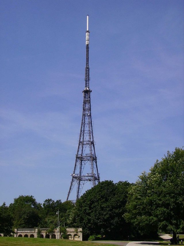
The Crystal Palace transmitting station mast
The audio signal itself occupies the frequency range 50 Hz - 15 kHz, which includes most of the frequencies we can actually hear. For a purely monophonic broadcast, the audio signal is used to modulate a high-frequency carrier. The upper modulating frequency is 15 kHz, and if we assume a maximum deviation of ± 75 kHz, we have a modulation index of 5.0 and a total bandwidth requirement (according to Carson's rule) of 180 kHz. In reality, as we shall see, things are somewhat more complicated, because most if not all FM radio stations broadcast in stereo, and often transmit supplementary programs and information signals in addition to the stereo broadcast itself.
Current transmission standards for FM sound broadcasting at VHF are specified in Recommendation ITU-R BS.450-4 (10/2019), published by the Radiocommunication Sector of ITU (ITU-R). This document describes the technical requirements for analogue FM sound broadcasting systems in Band 8 (the VHF radio frequency band). The BS in the title stands for broadcasting service. Specifically, it details the requirements for monophonic transmissions, stereophonic transmissions using a polar modulation system, and stereophonic transmissions using a pilot-tone system.
Pre-emphasis
In all three types of transmission, the baseband audio signal to be transmitted undergoes a process known as pre-emphasis before it is used to modulate the high frequency carrier. This process essentially boosts the signal power for frequencies at the upper end of the audio spectrum, where background noise can be heard as a faint but incessant hiss. At the receiver, the demodulated signal undergoes the reverse process (de-emphasis), which has the added benefit of reducing the background noise generated at the upper end of the audio spectrum in the receiver.
Pre-emphasis can itself be problematical because today's contemporary music tends to feature a greater proportion of high-frequency sounds than the kind of music broadcast in the early days of FM radio, and the pre-emphasis of these high-frequency sounds can lead to a frequency deviation in excess of the permitted maximum value.
This problem can be countered using a limiter – essentially, an electronic circuit that attenuates any signals whose amplitude exceeds some pre-defined threshold. This is a form of dynamic range compression (DRC) - a process that amplifies the quiet sounds in an audio signal, or reduces the volume of loud sounds in the signal, in order to compress its dynamic range (the difference in amplitude between the quietest and loudest sounds that make up the audio signal).
For monophonic transmission, the carrier is modulated by the pre-emphasised audio signal, with a maximum frequency deviation of either ± 50 kHz or ± 75 kHz (in most regions, including Western Europe and the United States, maximum frequency deviation is ± 75 kHz). Stereophonic transmission is a somewhat more complex process due to the need to multiplex (i.e. combine) two baseband signals - the left and right audio channels, designated as channels A and B respectively - into a single composite signal that can be used to modulate the high-frequency carrier.
Stereophonic transmission
As mentioned above, ITU-R defines two forms of stereophonic transmission. These differ in the way that channels A and B are multiplexed prior to the modulation process in order to produce what the standard refers to as the "stereophonic multiplex signal", i.e. the signal produced as a result of the multiplexing process. The standard also states, however, that stereophonic transmissions using a pilot-tone system "has become the de facto standard worldwide". Consequently, we will only examine this form of stereophonic transmission in this article.
The multiplexing process consists of the following steps:
- The audio frequency channels A and B are summed to create a monophonic baseband signal M. The amplitude of signal M is then reduced by 50%.
- Signal M is pre-emphasized as described above (alternatively, the pre-emphasis can be applied to channels A and B separately, before they are summed; the result will be the same).
- A second baseband signal S is created by subtracting channel B from channel A. The amplitude of signal S is also reduced by 50%.
- Signal S is pre-emphasized in the same way as signal M, and is then used for the suppressed-carrier amplitude modulation of a 38 kHz sub-carrier frequency, generating two sidebands.
- A pilot tone is generated at a frequency of 19 kHz (exactly one half of the sub-carrier frequency).
The illustration below is a simplified block diagram of the circuitry typically used to generate a stereophonic multiplex signal. Pre-emphasis of signals A and B (the left- and right-hand stereo signals) is performed using a pair of high-pass filters, and the pre-emphasized signals are sent to adder circuits. One adder circuit outputs the sum of the two signals (A + B) and the other outputs the difference (A – B).
The difference signal is sent together with a 38 kHz signal to a balanced AM modulator, which outputs a double-sideband suppressed carrier (DSB-SC) signal centred at 38 kHz. The 38 kHz signal is also passed through a frequency divider in order to create the 19 kHz pilot tone. All three signals are then sent to a second adder circuit, which sends the resulting multiplexed signal to the FM transmitter.
A basic FM stereo multiplexing circuit
Signal M and signal S are usually referred to as the sum and difference signals respectively. The stereophonic multiplex signal used to modulate the main carrier thus consists of signal M, the 19 kHz pilot tone, the two sidebands created by using signal S to amplitude modulate the 38 kHz sub-carrier, and the vestigial 38 kHz sub-carrier itself, as shown in the illustration below.
The stereophonic multiplex signal generated by a pilot-tone system
In a frequency modulated signal, the amplitude of the modulating signal is used to vary the frequency of the carrier around its nominal centre frequency. The maximum amplitude of the stereophonic multiplex signal used to modulate the carrier must therefore not exceed the level corresponding to the maximum frequency deviation (± 75 kHz). The maximum amplitude of each component of the stereophonic multiplex signal is limited to a percentage of this level as follows:
- Signal M: 90% (A and B being equal and in phase)
- Pilot tone: 8-10%
- Sum of signal S sidebands: 90% (A and B being equal and of opposite phase)
- Residual 38 kHz sub-carrier: 1%
The phase relationship between the 19 kHz pilot tone and the 38 kHz sub-carrier must be such that the unmodulated sub-carrier signal would cross the time axis with a positive slope each time the pilot signal has an instantaneous value of zero, with a tolerance of ± 3°.
The transmitted signal is compatible with monophonic receivers because all of the monophonic audio information is carried by signal M, which is the sum of channels A and B. The stereo information in the received signal is effectively filtered out after the incoming signal has been demodulated to recover the baseband stereophonic multiplex signal.
For stereo receivers, channels A and B can be recovered relatively easily from the baseband signal. The presence of the pilot tone tells the receiver that a stereo signal is being transmitted. The 19 kHz frequency of the pilot tone is then doubled by the receiver in order to re-create the 38 kHz sub-carrier. The sub-carrier is subsequently used to demodulate the double sideband signal and extract the difference signal S.
The left-hand channel (channel A) is recovered by adding the sum and difference signals M and S and dividing by two:
| A = | M + S | = | (A + B) + (A – B) |
| 2 | 2 |
The right-hand channel (channel B) is recovered by subtracting the difference signal S from the sum signal M and dividing by two:
| B = | M - S | = | (A + B) - (A – B) |
| 2 | 2 |
Supplementary programs and signals
As we can see from the foregoing, the bandwidth of the stereophonic multiplex signal - and hence the highest modulating frequency - is 53 kHz, which would give us a modulation index of 1.415 if we assume a maximum deviation of ± 75 kHz. However, it may have occurred to you that if we can embed a pilot tone and stereo information into the baseband signal, then it should be possible to embed additional channels or information signals. Indeed, this is often what happens.
Additional monophonic audio channels or data channels can be added to the baseband signal using additional sub-carriers. These channels, which cannot usually be received using standard radio equipment, can be used for a multitude of purposes, including paging services, stock market reports, messaging, background music, and foreign language programmes.
Note that the inclusion of additional channels is only permitted if compatibility with existing receiving equipment is maintained. The additional signals must not interfere with, or affect the quality of, the main monophonic or stereophonic programmes. Consequently, the sub-carrier frequency and its corresponding frequency deviation must be such that the instantaneous frequency of the signal is restricted to between 53 kHz and 76 kHz. The sub-carriers used for supplementary information signals must have a centre frequency of between 15 and 23 kHz, or between 53 and 76 kHz.
Most European FM broadcast services now transmit service-related digital information such as the time, the station ID, and program information using the Radio Data System (RDS), a communications protocol that can be used to embed a limited amount of digital information in the FM baseband signal. The sub-carrier used for this service has a frequency of 57 kHz - the third harmonic of the 19 kHz FM stereo pilot tone. This frequency was chosen in order to minimize interference between the pilot tone, the RDS signal itself, and the 38 kHz DSB-SC stereo difference signal (the maximum deviation of the RDS signal is typically between 2 and 4 kHz).
If the baseband signal used to modulate the main carrier does include additional programmes or supplementary information signals, and assuming a maximum frequency deviation of ± 75 kHz, then the monophonic or stereophonic signal is required to have an amplitude of not less than 90% of the maximum permitted value, and the additional signals are restricted to a maximum amplitude of 10% of that value. Under no circumstances may the maximum deviation of the main carrier by the total baseband signal exceed ± 75 kHz.
Direct generation of FM
An FM transmitter uses the baseband monophonic or stereophonic multiplex signal to modulate a VHF radio frequency carrier, amplifies the resulting signal, and broadcasts it. The FM signal itself can be generated either directly or indirectly (using phase modulation as an intermediate step), but we'll look first at the direct (or parameter variation) method, which generates an FM signal using a relatively straightforward oscillator circuit.
For direct FM, the baseband information signal is used to directly vary the oscillation frequency of a voltage-controlled oscillator (VCO), also known as a voltage-to-frequency converter (VFC). The instantaneous oscillation frequency output by the VCO depends on the instantaneous input voltage. The following block diagram illustrates the general principle.
Direct FM can be generated using a voltage-controlled oscillator (VCO)
The simplest type of voltage-controlled oscillator basically consists of an LC circuit (also known variously as a resonant circuit, tank circuit or tuned circuit) consisting of an inductor (L) and a capacitor (C) connected in parallel. The inductor and capacitor are chosen so that the inductive reactance and the capacitive reactance are of equal magnitude, which causes electrical energy to oscillate between the magnetic field of the inductor and the electric field of the capacitor.
The frequency of the oscillation depends on the resonant frequency of the LC circuit, which in turn depends on the values of the inductor and capacitor, according to the following formula:
| fc = | 1 |
| 2π√LC |
Where L is inductance and C is capacitance.
It should be clear from the above that varying the value of either the circuit's inductance or its capacitance will change the resonant frequency of the circuit. One simple way of achieving this would be to use a variable reactance device such as a varicap diode (also known as a varactor diode) as one of the elements of the VCO circuit. The reactance of the varicap diode is voltage dependent, so it can be used to vary the capacitance - and hence the resonant frequency - of the VCO circuit. This type of VCO is called a reactance modulator. The principle is illustrated below.
A typical VCO employs a variable reactance device coupled with an LC circuit
A VCO can be used to generate both narrowband and wideband FM signals, depending on the centre frequency and the Q factor of the VCO. In this context, the Q factor represents the ratio of the centre frequency of a resonant circuit and its bandwidth (the difference between the highest and lowest frequencies attainable). When a modulating signal m(t) is applied to the input of a VCO, the instantaneous frequency f(t) of the output signal can be expressed as:
f(t) = fc + kvco m(t)
where kvco is a constant that represents the oscillator sensitivity (or gain), of the VCO expressed, in hertz per volt, and kvco m(t) is the instantaneous frequency deviation.
Relatively high bandwidth VCOs are available as low-cost integrated circuits whose frequency will vary uniformly with respect to the input voltage, which would indicate that the VCO is an ideal choice for generating a wideband FM signal. There is a problem, however. Unlike a crystal oscillator, which has a highly stable resonant frequency, the resonant frequency of a VCO has a tendency to drift. For some applications this is not a problem, but in applications such as commercial radio broadcasting, where carrier frequencies are tightly constrained, it becomes necessary to somehow stabilise the centre frequency of the VCO.
The solution is to implement the VCO circuitry as a phase-locked loop (PLL) - a feedback system in which a phase comparator is used to compare the phase of the VCO's output signal with the phase of a reference signal. They are typically used to generate stable high-frequency signals, using a relatively low-frequency crystal oscillator to generate the reference signal. The crystal oscillator has a frequency fosc that is some fraction of the VCO's nominal centre frequency fc , such that:
fosc = fc / N
The output from the VCO is sent to a frequency divider that divides the frequency of the received signal by N. Both the output of the frequency divider and the output of the reference oscillator are then sent to a phase comparator. The phase comparator decides which of the two signals has the higher frequency by comparing the phases of both signals, and generates the appropriate error voltage, which is then added to the information signal and fed back to the VCO's input.
If the VCO frequency is higher than the reference frequency, the error voltage is reduced in order to slow the VCO down until the phases of the two signals arriving at the inputs to the phase comparator are the same. If the VCO frequency is lower than the reference frequency, the error voltage is increased in order to speed the VCO up until the phases are the same. The output frequency of the VCO is thus stabilised by phase-locking its operating frequency to that of the crystal oscillator. A block-diagram of a basic PLL-stabilised VCO is shown below.
A phase-locked loop is used to stabilise the centre frequency of a VCO modulator
Something may have occurred to you after reading the above description. The output frequency of the VCO at any given time depends on the voltage of the signal arriving at the VCO's input, but the feedback loop is compensating for frequency drift by adjusting the error voltage so as to "iron out" any variation in the VCO's output frequency. This would, of course, include the variation caused by the modulating signal itself.
However, any variation in the error voltage due to a drift in the centre frequency of the VCO will be gradual, and thus have a relatively low frequency, whereas the variation in the error voltage due to the modulating signal will reflect the voltage variations in the modulating signal itself, and will have frequencies in the audio range. We therefore use a low-pass filter to remove these higher frequencies from the error voltage before it reaches the mixer, leaving just the underlying trend.
Indirect generation of FM
Direct FM is relatively easy to implement for applications where frequency drift is not a problem, but in wideband applications such as commercial FM radio where strict regulatory requirements apply, the need to stabilise the carrier frequency significantly increases the complexity of the modulator circuitry, making it both more difficult to implement and more expensive. An alternative approach is to produce wideband FM indirectly.
This is typically achieved by integrating the modulating signal and sending it to a narrow band phase modulator (we saw above how the relationship between phase and frequency makes this possible). The output of the phase modulator will be a narrow band FM signal, so a series of mixers and frequency multipliers are then used to increase the frequency and bandwidth of the FM signal until the required centre frequency and modulation index are reached. The illustration below is a simplified block diagram of how an indirect wideband FM signal is generated.
A block diagram showing the indirect method of generating wideband FM
This method of generating wideband FM is sometimes referred to as the Armstrong method after the American electrical engineer and inventor Edwin H. Armstrong (1890 - 1954), who first developed the idea. The main advantage of this method is that it uses a highly stable crystal oscillator to generate the carrier, so frequency stabilisation is not an issue. The downside is that frequency deviation is usually limited to values of under one kilohertz in order to avoid signal distortion. As we have seen, narrow band FM typically has a peak deviation of ± 5 kHz, and commercial FM radio requires ± 75 kHz. Frequency multipliers are therefore required in order to achieve the required bandwidth.
We'll come back to the topic of frequency multipliers in due course. First, we'll look at how the narrow band phase modulator works. Consider the block diagram below, which shows the narrow band phase modulator in more detail.
Block diagram showing indirect method of generating wideband FM
The product modulator receives two inputs - the integrated information signal, and the carrier signal generated by the crystal oscillator, phase shifted through -90° (-π/2 radians) by the phase shifter.
We saw earlier that if the modulating signal m(t) has a sinusoidal waveform, it can be expressed as:
m(t) = Am cos(2πfm t)
where Am is the maximum amplitude of the modulating signal and 2πfm is its frequency. Integrating the modulating signal with respect to time will therefore give us:
| ∫ | t | Am cos(2πfm t) dt = | Am | sin(2πfm t) |
| 0 | 2πfm |
The output from the integrator will be a signal voltage whose amplitude is proportional to the integral of the modulating signal. The integrator itself is usually implemented using a special kind of operational amplifier (or op-amp), but the amplitude of the output signal will probably be significantly smaller than that of the input signal, depending on the characteristics of the op-amp. And, while the output signal has the same frequency as the modulating signal, it is out of phase with it by -2π radians (-90°).
Before we proceed, we should probably look at how a typical narrowband phase modulator actually works. This includes taking a more detailed look at the product modulator. This type of modulator takes two inputs - a high frequency carrier and a lower frequency modulating signal - and generates a double sideband suppressed carrier (DSB-SC) as its output. The product modulator - also known as a DSBSC modulator for obvious reasons - is so called because the signal it outputs is the product of the two input signals.
There are different ways of implementing a product modulator, all of which achieve more or less the same result. The type of product modulator we're going to look at here is called a balanced modulator, because it actually consists of two identical amplitude modulators, each of which produces an amplitude modulated signal at its output, in a balanced configuration. The purpose of this arrangement, which is illustrated in the block diagram below, is to remove the carrier signal after the modulation has taken place.
Block diagram of a balanced modulator
Product modulators are so called because the operations they carry out essentially involve multiplying two signals together in some way. In a balanced modulator, each AM modulator multiplies the carrier signal by one plus a value that is proportional to the modulating signal. That value is calculated as the product of the modulating signal and some constant scaling factor, which we'll call ka . Thus, if we call the output of the upper modulator s1 (t) and the output of the lower modulator s2 (t), we can express the resulting AM signals as follows:
s1 (t) = Ac cos(2πfc t) [1 + ka m(t)]
s2 (t) = Ac cos(2πfc t) [1 - ka m(t)]
At the mixer, signal s2 (t) will be subtracted from signal s1 (t), and its output will be a DSB-SC signal, s(t), that is calculated as follows:
s(t) = Ac cos(2πfc t) [1 + ka m(t)] - Ac cos(2πfc t) [1 - ka m(t)]
s(t) = Ac cos(2πfc t) 2ka m(t)
As stated above, a balanced modulator essentially takes two signals - the modulating signal and the carrier - and multiplies them together. Accordingly, the standard equation of a DSB-SC signal is:
s(t) = Ac cos(2πfc t) m(t)
If we compare this equation with the expression we arrived at for the output of our balanced modulator, we can see that there is an overall scaling factor of 2ka . This value determines the bandwidth of the DSB-SC signal, and its significance will be seen when we look at how the output of the product modulator is used in a narrow band phase modulator to produce an FM signal.
Let's now consider what is happening in the narrow band phase modulator. The first thing to note is that the modulating signal is passed through an integrator before it is sent to the product modulator, so the output of the phase modulator will essentially be a frequency modulated signal.
The second thing to note is that, although the carrier signal from the crystal-controlled oscillator is sent to both the product modulator and the mixer, the carrier signal supplied to the product modulator is phase-shifted through -2π radians (-90°). This means that the output of the product modulator will be 90° out of phase with the unshifted carrier. If this were not the case, the output of the phase modulator would be an amplitude modulated signal instead of a narrow band FM signal.
We'll start by re-writing the expressions for the outputs of the upper and lower modulators modulator, s1 (t) and s2 (t):
| s1 (t) = Ac sin(2πfc t)[1 + ka | ∫ | m( t)] |
| s2 (t) = Ac sin(2πfc t)[1 - ka | ∫ | m( t)] |
As we have seen, the output of the product modulator will be the result of subtracting signal s2 (t) from signal s1 (t) to produce a phase-shifted DSB-SC signal, s(t). Here is the revised calculation:
| s(t) = Ac sin(2πfc t)[1 + ka | ∫ | m( t)] | - Ac sin(2πfc t)[1 - ka | ∫ | m( t)] |
| s(t) = Ac sin(2πfc t) 2ka | ∫ | m( t) |
The output of the mixer will be a narrowband FM signal, sFM (t), that is the sum of the unshifted carrier and the phase-shifted DSB-SC signal:
| sFM (t) = Ac cos(2πfc t) + Ac sin(2πfc t) 2ka | ∫ | m( t) |
If we expand the expression for the integral of m(t), we get:
| sFM (t) = Am cos(2πfc t) + Ac sin(2πfc t) | ka Am | sin(2πfm t) |
| πfm |
The FM modulation index
You may have noted that the equation for the narrowband FM signal sFM (t) (see above) contained the fractional term:
| ka Am | |
| πfm |
This term represents the modulation index, β, for the FM signal. As we have mentioned previously, the FM modulation index is defined as the ratio of the frequency deviation (Δf) to the modulating frequency (fm ):
| β = | Δf |
| fm |
Note that the term ka here equates to the term kf which, as we saw earlier, is one of the terms used to define the instantaneous frequency f(t) of a frequency modulated signal. It represents the frequency sensitivity, i.e. the amount by which the frequency of the carrier will vary in response to a variation in the amplitude of the modulating signal:
f(t) = fc + kf m(t) = fc + kf Am cos(2πfm t)
In the simple case of a sinusoidal modulating signal, all of the terms that make up the modulation index will be constant, but if a complex audio waveform is used to modulate the carrier (this will normally be the case), then things get a little more complicated, because both the frequency and maximum amplitude of the modulating signal will vary. Thus, when the modulating signal is a complex audio wave, the modulation index is usually calculated using the maximum frequency deviation and the highest audio frequency.
The resulting value will be used to derive the peak deviation (see above) of the frequency modulated signal, from which its bandwidth requirements can subsequently be determined (using Carson's rule, for example). Whichever calculation is used, it should be noted that none of the terms in the modulation index include the carrier frequency, which means that the modulation index is independent of the carrier frequency.
In order to comply with our (very broad) definition of narrow band FM, the value of β must be limited to ≤1, and is typically around 0.3. It is also necessary to limit the value of β in order to minimise any distortion that may occur within the phase modulator. It is therefore obviously not possible to generate wideband FM directly, since this would require a much higher modulation index - at least 1.0, and usually higher, depending on the application.
Bear in mind also that the carrier frequency generated by the crystal oscillator is usually only a fraction of the carrier frequency required by most commercial applications. We need a way of increasing the both the modulation index and the carrier frequency to the required levels. This means passing the narrow band FM signal through a sequence of frequency multipliers and mixers.
A frequency multiplier increases the modulation index and carrier frequency by multiplying the FM signal carrier by some factor, which we'll call n. Consequently, both the carrier frequency and the frequency deviation of the FM signal will increase n-fold. Since the frequency of the modulating signal itself is not affected by the frequency multiplier, the value of the modulation index also increases n-fold (remember that β = Δf/fm ).
There is, however, a potential problem here because Armstrong's indirect method of generating an FM signal only produces a very small frequency deviation - the peak deviation is typically only a very small fraction of 1 kHz. A typical FM voice channel requires a maximum frequency deviation of 5 kHz, and a commercial FM broadcast channel requires a peak deviation of ± 75 kHz.
Frequency multipliers and mixers
Let's consider an Armstrong NBFM generator that obtains its carrier signal from a 200 kHz oscillator, and produces a maximum frequency deviation of 25 Hz. Let's assume that we want to produce a wideband FM signal with a carrier frequency is 90 MHz and a peak deviation of ± 75 kHz. In order to achieve our peak deviation target for the wideband FM signal, we could simply multiply the NBFM signal by 3,000 (75,000 ÷ 25 = 3,000). However, since the carrier frequency would also be multiplied by 3,000, we would end up with a carrier frequency of 600 MHz (3,000 × 200,000 = 600,000,000) many times higher than we actually require.
We need to find a way of increasing both the peak deviation and the carrier frequency to the correct levels, which means that frequency multipliers alone are not the answer. That is where mixers come to the rescue. A mixer adds two input signals together to produce two new signals - the sum and the difference of the two input signals. A bandpass filter at the mixer's output determines whether the mixer outputs the sum or the difference signal. The important thing to note here is that the mixer can increase or decrease the carrier frequency without changing the frequency deviation. Consider the block diagram below.
Multipliers and mixers are used to achieve the required carrier frequency and modulation index
The signal leaving the Armstrong FM modulator has a centre frequency f1 = 200 kHz and a maximum frequency deviation Δf1 = 25 Hz. The signal is sent to a frequency multiplier with a multiplication factor of 60. The resulting signal is then sent to a mixer whose second input comes from a stable 10.2 MHz local oscillator (we will work on the assumption that the filter at the oscillator's output will filter out any frequencies in excess of this value). The output from the mixer is then sent to a second frequency multiplier, this time with a multiplication factor of 50. What centre frequency and peak deviation will our wideband signal have?
The first frequency multiplier produces an output signal with a centre frequency f2 and a maximum frequency deviation Δf2 :
f2 = f1 × 60 = 200 kHz × 60 = 12 MHz
Δf2 = Δf1 × 60 = 25 Hz × 60 = 1.5 kHz
The output from the mixer will be the difference of the two input signals. It will have a centre frequency f3 and a maximum frequency deviation Δf3 = Δf2 = 1.5 kHz. Frequency f3 is the result of the following frequency conversion:
f3 = f2 - 10.2 MHz
f3 = 12 MHz - 10.2 MHz
f3 = 1.8 MHz
The output of the mixer is sent to the second multiplier, resulting in a wideband FM signal with centre frequency f4 and peak deviation Δf4 , calculated as follows:
f4 = f3 × 50 = 1.8 MHz × 50 = 90 MHz
Δf4 = Δf3 × 50 = 1.5 kHz × 50 = 75 kHz
We have thus achieved the required centre frequency and peak deviation for the wideband FM signal to be transmitted. Keep in mind, however, that commercially available frequency multipliers tend to have relatively low multiplication factors, typically ranging from ×2 up to ×10, so real world wideband FM transmitters tend to use several multipliers in series on either side of the mixer in order to achieve the required carrier frequency and peak deviation.
The FM receiver
The job of the FM receiver is to detect the incoming FM signal, amplify and demodulate it, and convert the resulting audio signal into an audible audio output using a suitable transducer (e.g. a loudspeaker or headset). A simplified block diagram of an FM receiver is shown below.
A simplified block diagram of an FM receiver
In the FM receiver, a number of distinct stages are involved in converting the incoming FM signal into a baseband audio signal. The first stage takes place when the antenna receives the incoming radio frequency signals. Because these signals are typically very weak, they are passed to an RF amplifier. A tuner is used to select the required carrier frequency and filter out any signals that do not fall within the selected FM band.
The amplified RF signal is then sent to the mixer, which receives a relatively low-frequency sinusoidal signal from a local oscillator as its second input. The mixer adds the incoming RF signal to the oscillator signal to produce an intermediate frequency (IF) signal. Lowering the frequency of the signal (in practice, this can be done in several stages) has several benefits, one of which is that the filters used to eliminate unwanted signals tend to function more effectively at lower frequencies.
After leaving the mixer, the incoming signal is again amplified, this time by an IF amplifier. This essentially works in the same way as the RF amplifier, but for lower frequencies. The amplified signal is then sent to the FM demodulator, which must detect the frequency variations in the IF signal and translate these into the amplitude variations of an audio frequency signal. The audio frequency signal is then amplified by the AF amplifier and sent to a transducer (usually a loudspeaker) which creates the audio output.
As we have mentioned, the demodulator's job is to convert the radio frequency FM signal into an audio frequency signal - essentially, the same audio frequency signal that was used by the transmitter to modulate the RF carrier in the first place. Various kinds of circuit can be used to demodulate the FM signal, including:
- Slope detectors
- Foster-Seeley discriminators
- Ratio detectors
- Phase-locked loop (PLL) FM detectors
- Quadrature FM detectors
The first three circuits are all built using discrete electronic components and are not suited to implementation as part of an integrated circuit. The simplest of these is the slope detector which we'll look at in some detail. We'll also look at the Foster-Seeley discriminator, which gives better overall performance but is somewhat more complex. The ratio detector is essentially a variant of the Foster-Seeley discriminator, so we'll leave it for the interested reader to investigate.
The last two circuits on our list can both be found in in modern radio receiving equipment because they are well suited to implementation as part of an integrated circuit, although the quadrature FM detector also requires the use of an inductor coil. This is not generally considered to be a major disadvantage since a relatively inexpensive coil can be used, but we'll be concentrating our efforts on describing the operation of the phase-locked loop FM detector, which can be implemented without using discrete components. Again, we leave it to the interested reader to investigate the operation of the quadrature FM detector.
The slope detector
This is a very simple, although not particularly effective, method that was widely used in the early days of FM radio. The slope detector (also known as a frequency discriminator) typically consists of a tuned transformer with a resonant frequency that is slightly offset from the carrier frequency. The response of the tuned circuit will vary with the frequency of the incoming signal, so its output is essentially a frequency modulated signal that is also amplitude modulated. This FM/AM signal is then applied to a simple diode envelope detector circuit - essentially a half-wave rectifier coupled with a low-pass filter - that removes the high-frequency carrier and recovers the baseband information signal. The diagram below illustrates the principle.
Block diagram of a slope detector FM demodulator
The resonant frequency must be offset from that of the carrier because, as the carrier frequency approaches that of the tuned LC circuit, the amplitude of the resulting AM signal will rise; as it gets farther away from the carrier, the amplitude of the AM signal falls. The offset must be sufficiently large (usually several hundred kilohertz) that the frequency of the modulated carrier never exceeds that of the tuned circuit.
The circuit shown above is one of several configurations that could be used. The frequency modulated input signal is applied to a tuned circuit consisting of transformer T1 and capacitors C1 and C2. The resulting amplitude modulated FM signal is then applied to the envelope detector circuit. Diode D1 rectifies the AC signal, while capacitor C3 removes the unwanted high frequency components. Resistor R1 provides a load.
The main advantage of this kind of FM demodulator is that it is relatively easy to implement, but there are a number of drawbacks. The response of the tuned circuit will not be linear, which will inevitably lead to some distortion of the amplitude modulated signal. The resonant frequency of the LC circuit must be carefully chosen to ensure that its response curve is as linear as possible, in order to minimise the distortion.
Another problem is that, because the slope detector essentially converts the incoming signal to an AM signal, any variations in the amplitude of the FM signal will appear as noise at the output. Such variations in amplitude can be mitigated to a large extent by using an amplitude limiter circuit on the incoming signal before it reaches the detector, although this will increase the complexity of the receiver.
We should also consider the fact that, because the response of the detector varies with the frequency of the incoming FM signal, and will never quite attain its maximum value, the FM signal can never be received at its maximum signal strength. Added to the other limitations associated with this demodulation method, it is not hard to see why it is no longer widely used, although it is useful to have an understanding of the underlying concepts involved.
The Foster-Seeley discriminator
Invented in 1936 by Dudley E. Foster and Stuart William Seeley, the Foster-Seeley discriminator - also known as the phase shift discriminator - is a type of FM demodulator that was widely used when radio receivers were built using discrete components and, like the slope detector and the ratio detector, it is no longer widely used. The circuit consists of capacitors, resistors, diodes, an RF transformer, and an RF choke. The diagram below shows a basic Foster-Seeley discriminator circuit.
A basic Foster-Seeley discriminator circuit
Like the slope detector we saw above, the Foster-Seeley discriminator incorporates a tuned transformer circuit, but that's pretty much where the similarity ends. We can think of it as two LC circuits (you may also see these described as tank circuits, resonant circuits or tuned circuits). The primary LC circuit comprises the transformer's primary winding L1 and capacitor C1, and the secondary LC circuit comprises the transformer's secondary winding and capacitor C2. Note that the secondary winding has a centre tap which is effectively at ground potential. We can therefore think of it as two separate inductors, which we have labelled L2 and L3. Both LC circuits are tuned to the incoming FM signal's centre frequency.
A connection is made from the primary LC circuit to the centre tap on the secondary winding via capacitor C3, which acts as a coupling capacitor (i.e. it allows high frequency AC signals to pass through it while blocking low frequency AC and DC signals). The centre tap is also connected to RF choke L4, which is thus effectively in parallel with the primary winding. An RF choke is an inductor that blocks high-frequency AC signals but allows low-frequency and DC signals to pass (an ideal RF choke only allows DC signals to pass).
Together with capacitors C4 and C5, the choke prevents any RF signals from appearing at the output of the discriminator. It also acts as a return path for the DC current leaving diodes D1 and D2. As we saw in the simple slope detector above, each diode-capacitor pairing (D1-C4 and D2-C5) forms an envelope detector circuit consisting of a half-wave rectifier and low-pass filter. Resistors R1 and R2 are the load resistors for diodes D1 and D2 respectively.
The Foster-Seeley discriminator circuit is not the easiest of circuits to understand. We'll attempt to explain it in a non-mathematical way, but it will be necessary to refer to the relevant phasor diagrams in order to gain a basic understanding of how it works. In these diagrams, the input voltage Ep applied to primary winding L1, which also appears across RF choke L4, is used as a reference voltage, and is drawn as a horizontal vector pointing to the right, away from the origin. We present below the relevant phasor diagrams.
Phasor diagrams: (a) at resonance, (b) above resonance and (c) below resonance
The phasor diagrams represent three possible scenarios. In the first scenario (a), the incoming signal is at the centre (i.e. resonant) frequency, which will be the case when there is no modulating signal (or the modulating signal is instantaneously passing through the zero axis). In the second scenario (b), the modulating AF signal has a positive voltage, and the frequency of the incoming FM signal is higher than the centre frequency. In the final scenario (c), the modulating AF signal has a negative voltage, and the frequency of the incoming FM signal is lower than the centre frequency.
Before we look at what is happening in each of these scenarios, let's consider what we can deduce by studying these phasor diagrams in conjunction with the circuit diagram:
- Primary input voltage Ep is applied to both diode D1 and diode D2, because one end of L4 is connected to the cathode of each diode via a load resistor, and the other end is connected to the anode of each diode via the secondary winding.
- E1 and E2 represent the reactive voltages across inductors L2 and L3 respectively. They will always be out of phase with Ep (the voltage across L4) by some margin.
- E3 and E4 represent the total voltages applied to diodes D1 and D2 respectively. E3 is the vector sum of the voltages across L2 and L4, i.e. the vector sum of E1 and Ep . Similarly, E4 is the vector sum of the voltages across L3 and L4, i.e. the vector sum of E2 and Ep .
- Reactive voltages E1 and E2 have opposite polarities with respect to the centre tap on the secondary winding, and are thus always 180° out of phase with each other.
- Reactive voltages E1 and E2 are always 90° out of phase with the secondary current. E1 always leads Is by 90°, while E2 always lags Is by 90°.
- Voltages E3 and E4 always have opposite polarity regardless of variations in frequency, but at resonance they will have equal magnitude.
- Above resonance, the phase difference between E3 and Ep is reduced while the phase difference between E4 and Ep increases, resulting in voltage E3 having a greater magnitude than voltage E4 .
- Below resonance, the phase difference between E3 and Ep increases while the phase difference between E4 and Ep is reduced, resulting in voltage E4 having a greater magnitude than voltage E3 .
Circuit operation at resonance:
We'll look first at how the circuit behaves when the incoming signal is at the centre frequency, i.e. unmodulated. The current through any coil lags the voltage across it by 90°, so the current Ip in the primary winding lags primary voltage Ep by 90°. This primary current induces a voltage in the secondary winding and, since this voltage will be greatest when the primary current is changing at the fastest rate, i.e. when it passes through the zero axis, the induced secondary voltage is 90° out of phase with the primary current.
Since the primary current is 90° out of phase with both primary voltage Ep and the induced secondary voltage, then the induced secondary voltage must either be in phase or 180° out of phase with Ep . We will work here on the assumption that these voltages are in phase (note that, according to some sources, primary and secondary voltages are 180° out of phase, although it depends on the direction in which the transformer coils are wound with respect to one another. The distinction is not particularly significant with respect to how the Foster-Seeley discriminator actually works).
The secondary voltage generates a current Is in the secondary coil. Because the secondary LC circuit is resonant at the centre frequency, the inductive reactance and the capacitive reactance in the circuit cancel each other out, so it acts like a resistive circuit. In a resistive circuit, current is in phase with the voltage that drives it, so secondary current Is is in phase with the induced secondary voltage, and therefore is also in phase with Ep as shown in phasor diagram (a). However, because the secondary winding is an inductor, the current flowing through it generates a reactive voltage across it that is 90° out of phase with Is (and therefore also 90° out of phase with Ep ).
Because E1 and E2 are 180° out of phase with each other and 90° out of phase with Ep , the voltages applied to diodes D1 and D2, i.e. the vector sums E3 and E4 respectively, will have the same magnitude but opposite signs. This means, in essence, that each diode conducts the same amount of current, but on alternate half cycles of the input waveform. The output from each diode is basically a stream of DC pulses at the RF rate which will be "smoothed out" by capacitors C4 and C5 to produce varying DC voltages across resistors R1 and R2. Since these voltages are equal in magnitude but opposite in polarity, they cancel each other out and there is no AF output.
Circuit operation above resonance:
When the frequency of the incoming signal is higher than the centre frequency, the secondary LC circuit no longer acts like a resistive circuit. In any LC circuit operating at the resonant frequency, the inductive reactance and the capacitive reactance are equal and effectively cancel each other out. As frequency increases beyond the resonant frequency however, inductive reactance increases and capacitive reactance is reduced, and the circuit becomes increasingly inductive in nature.
The secondary LC circuit now acts like an inductor, and secondary current Is lags primary voltage E p, as shown in phasor diagram (b). Since reactive voltages E1 and E2 must remain 90° out of phase with Is , E1 moves closer to being in phase with Ep while E2 becomes more out of phase with Ep . This results in an increase in the magnitude of vector sum E3 and a reduction in the magnitude of vector sum E4 . Diode D1 therefore conducts more than diode D2, and the voltage drop across resistor 1R is greater than that across resistor R2. The result is a positive DC voltage at the discriminator output that is proportional to the positive frequency deviation of the FM signal.
Circuit operation below resonance:
When the frequency of the incoming signal is lower than the centre frequency, the equilibrium between the inductive reactance and the capacitive reactance in the secondary LC circuit is once again lost. As the input frequency falls away from the resonant frequency, capacitive reactance increases and inductive reactance is reduced, and the circuit becomes increasingly capacitive in nature.
The secondary LC circuit now acts like a capacitor, and secondary current Is leads primary voltage Ep , as shown in phasor diagram (c). Since reactive voltages E1 and E2 must remain 90° out of phase with Is , E1 becomes more out of phase with Ep while E2 moves closer to being in phase with Ep . This results in a reduction in the magnitude of vector sum E3 and an increase in the magnitude of vector sum E4 . Diode D2 therefore conducts more than diode D1, and the voltage drop across resistor R2 is greater than that across resistor R1. The result is a negative DC voltage at the discriminator output that is proportional to the negative frequency deviation of the FM signal.
Summary
From the above, we can see that if the frequency of the incoming FM signal is greater than the centre frequency, there will be a positive DC voltage at the output of the discriminator that is proportional to the positive frequency deviation in the FM signal and therefore also proportional to the positive modulating signal voltage that generated it. Similarly, if the frequency of the FM signal is lower than the centre frequency, there will be a negative DC voltage at the output that is proportional to both the negative frequency deviation in the FM signal and the negative modulating signal voltage.
The two envelope detectors formed by diode-capacitor pairings D1-C4 and D2-C5 essentially reconstruct the positive and negative components respectively of the original audio frequency modulating signal. The illustration below shows a typical discriminator response curve.
A typical Foster-Seeley discriminator response curve
The Foster-Seeley discriminator provides good performance and a reasonably linear response over the range of frequencies it is designed for. It is also fairly easy to construct using discrete electronic components, and was once widely used in the manufacture of FM receiving equipment. Its main disadvantage is that it is sensitive to variations in signal amplitude, which translates into noise at the output. This problem can be mitigated by adding a special limiter circuit before the discriminator that limits the amplitude of the incoming signal to a prescribed level, although this adds complexity to the receiver and increases cost. Small amplitude variations not caught by the limiter circuit can still find their way to the discriminator output.
The phase-locked loop (PLL) demodulator
The phase-locked loop (PLL) demodulator has been widely used in radio receiving equipment since the advent of cheap, mass-produced integrated circuits. It provides good performance, even when the signal-to-noise ratio (SNR) is low, and is easy to implement within an integrated circuit. Few additional discrete components are required, and the need for wound components - always a major cost factor - has been eliminated altogether. The PLL demodulator tracks the instantaneous frequency of the incoming FM signal using a voltage-controlled oscillator (VCO). The illustration below is a block diagram of a basic PLL FM demodulator.
A basic phase-locked loop FM demodulator
As you can see from the diagram, the PLL FM demodulator consists of three major components - a phase detector (or phase comparator) a voltage-controlled oscillator (VCO), and a low-pass filter. The signal arriving at the demodulator has already been down-converted from a high frequency FM signal to an intermediate frequency (IF) signal using a mixer, usually in several stages. The most commonly used intermediate frequency for FM broadcast receivers appears to be 10.7 MHz, although other frequencies may be used.
Down-shifting the frequency of incoming FM signals is done for several reasons. Perhaps the most important of these is that, in order to select the required channel, a filter must be used. Since filter bandwidth tends to increase with frequency, low-frequency filters are far more selective than high-frequency filters. Shifting the selected FM channel to a fixed IF also means that the demodulator always operates at the same centre frequency, regardless of which channel has been selected. This simplifies signal processing, and makes it easier to design and build the demodulator circuitry.
The phase detector consists of a multiplying circuit or mixer that receives two input signals and multiplies them together. The output is a signal that contains two distinct frequency components - one at the sum of the input frequencies, and one at the difference of the input frequencies. It is the low frequency difference signal we are interested in here, since it will proportional to the phase difference between the two input signals.
A phase detector outputs the sum and difference of its input frequencies
The output from the LPF is usually referred to as the error signal. It serves as the control voltage for the voltage-controlled oscillator (VCO), which produces an output signal with an instantaneous frequency that is proportional to the control voltage.
In the PLL FM demodulator, one of the inputs to the phase detector is the downshifted FM signal, and the other is the output of the VCO. When there is no FM input to the PLL, it is said to be operating in free running mode. In this mode, the phase detector and LPF outputs will be zero, as will the VCO control voltage. The VCO itself is adjusted so that, in the free running mode, its output frequency will be identical to that of the unmodulated IF carrier. The VCO output will also be in phase quadrature (90° out of phase) with the unmodulated carrier.
Once the PLL starts to receive a modulated signal, it goes into capture mode. The difference signal generated by the phase detector will be proportional to the phase difference between the modulated signal and the VCO output, and because it is a relatively low-frequency signal will be allowed to pass by the LPF. The output of the LPF is a varying DC voltage that is fed back to the VCO input, causing the VCO to adjust its output frequency accordingly.
If the modulated carrier frequency is higher than the centre frequency, the error signal voltage will be positive, causing the VCO to increase the frequency of its output until it restores the 90° phase difference with the modulated input. Conversely, if the modulated carrier frequency is lower than the centre frequency, the error signal voltage will be negative, causing the VCO to reduce the frequency of its output in order to restore the 90° phase difference.
Once the required frequency and phase relationships have been achieved, the PLL is said to be in phase-locked mode. The PLL will then track changes in the input frequency and constantly adjust the error signal voltage in order to keep the VCO output in phase-lock with the modulated signal. The error voltage produced at the output of the error amplifier is proportional to the deviation of the input frequency from the centre frequency, and thus reproduces the original modulating signal.
The phase-locked loop typically has a wide bandwidth - usually much wider than the range of frequencies over which it is required to operate. It also has a high degree of linearity, depending on the VCO's voltage to frequency curve, which is typically very linear over the demodulator's operating range. For these and other reasons outlined previously, the PLL FM demodulator is a popular choice for FM radio receiving equipment.