Electromagnetic Waves
Overview
A wave can be defined as the transfer of energy between two points without any physical transfer of matter. Think about waves on the surface of the ocean. Although the surface of the water can be seen to rise and fall, the water itself tends to stay in one place. The energy carried by the waves, however, is a major factor in both coastal erosion and the deposit of materials on the shoreline.

Sound waves are waves that we can hear, and are caused by vibrating air molecules. The louder the sound, the more energy is being transferred. This can sometimes become painfully obvious, and in extreme cases can even cause physical damage. The noise from an explosion, for example, can damage your ears and may even cause permanent hearing loss. In fact, the energy in sound waves is used to good effect in lithotripsy, a medical procedure that breaks large kidney stones into smaller pieces.
Ocean waves and sound waves are examples of mechanical waves, so called because they involve the oscillation of some form of matter, and require some physical medium through which to propagate. Sound waves, for example, can propagate through both air and water, but they cannot propagate through a vacuum. They also diminish significantly in strength over relatively short distances (a process known as attenuation), and propagate at a relatively low speed (just under 350 metres per second).
All of which means that mechanical waves - even sound waves - are not a good option when it comes to communicating over long distances. Verbal communication is absolutely fine when we are in close proximity to other people. We could probably even communicate verbally over greater distances, either by shouting or by using a sound-amplifying device like a megaphone, but it wouldn't be very practical. Fortunately, we have learnt to harness the properties of electromagnetic waves for the purpose of long-distance communication.
Electromagnetic waves propagate very fast. The actual speed will depend on the transmission medium used but for guided media such as twisted pair copper cable or optical fibre, propagation speeds are typically between sixty percent and seventy-five percent of the speed of light in a vacuum. For unguided media such as radio or microwave transmissions, the propagation speed in Earth's atmosphere will approach that of light, although variations in atmospheric density and temperature will inevitably cause some refraction (bending) of the waves, which will slightly reduce the overall speed of propagation.
Electromagnetic waves can propagate over immense distances. The electromagnetic spectrum includes visible light, so when you look up at the stars in the night sky you are looking back in time. The light from the nearest star system (Alpha Centauri) has taken nearly four and a half years to reach Earth, even travelling at the speed of light, which is approximately 300,000 kilometres per second. And the light from some of those stars has taken many thousands of years to get here!
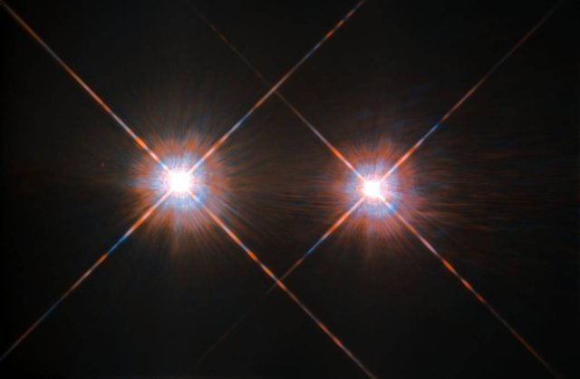
Hubble telescope image of Alpha Centauri A and B (4.37 light years from Earth)
Image credit: ESA/NASA
There are a vast range of frequencies available in the electromagnetic spectrum. The frequency of an electromagnetic wave represents the number of complete cycles a wave completes per unit time. The portion of the electromagnetic spectrum that can be used for radio transmission ranges from around 20 kilohertz (that's twenty thousand wave cycles per second) up to 300 gigahertz (three hundred thousand million wave cycles per second).
Although that sounds like an awful lot of bandwidth (the term bandwidth in this context refers to the range of frequencies available), bear in mind that not all of this bandwidth can be put to practical use. Some frequency ranges present challenges in terms of producing cost-effective and power-efficient telecommunications devices that can employ them, while other frequency ranges are simply too vulnerable to interference to be useful. And the demand for bandwidth increases daily. Apart from anything else, there are already (at the time of writing) some three-and-a-half billion smartphone users in the world!
On the other hand, it is now possible to run a home network over the electrical wiring used to distribute electricity to the power sockets in your home using a relatively low-cost and readily available Powerline networking solution. Given that these cables are often subject to a considerable amount of electrical "noise" that's a remarkable technical achievement in itself. Much of our telecommunications still relies, in fact on guided media in the form of copper cabling of one form or another, or on optical fibres.
Regardless of whether the transmission medium used is guided or unguided, virtually all telecommunication today depends on the transmission of electromagnetic waves from a transmitter to a receiver. The transmitted signals may consist of radio waves, microwaves, infrared light, or visible light. Electromagnetic waves at the higher and of the electromagnetic spectrum (i.e. with a frequency higher than that of visible light) include ultra violet light, x-rays, and gamma-rays. They are not used in telecommunications systems because they are potentially harmful to humans (the higher the frequency, the more potentially dangerous they become).
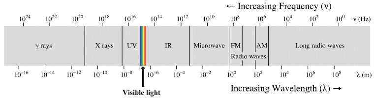
The electromagnetic spectrum
The information being transmitted over some transmission medium uses the electromagnetic wave as a carrier. The information is encoded for transmission by varying one or more of the physical properties of the carrier wave, such as its frequency, amplitude or phase (we'll be looking at these properties in more detail in due course), or some combination thereof. Both the type of electromagnetic wave used to carry a signal and the type of encoding used for the signal will depend on several factors, the most important of which is the nature of the physical transmission medium itself.
What is an electromagnetic wave?
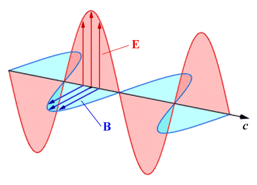
Before we talk about the properties of electromagnetic waves, we should probably establish what exactly an electromagnetic wave is. We know it's a wave (the name is a bit of a giveaway), and it's obviously got something to do with both electricity and magnetism - but how do these things relate to one another? The first thing to establish here is that an electromagnetic wave is actually a combination of two different waves.
Electromagnetic fields are created when moving charged particles such as protons or electrons generate a magnetic field, which interacts with the electric field surrounding static charged particles. Electromagnetic waves are oscillations of these fields that are in phase with one another, but which operate in planes that are perpendicular to one another. The electromagnetic wave propagates in a direction that is perpendicular to both of these planes (for this reason, it is said to be a transverse wave). The following diagram illustrates the principle:
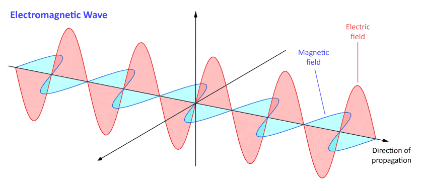
An electromagnetic wave consists of two perpendicular waveforms in phase with one another
Electromagnetic waves can propagate through solid materials, liquids, and gases in the same way as mechanical waves. Unlike mechanical waves, however, they can also propagate through a vacuum. They don't actually need a medium through which to propagate, because the changing electrical field component induces a similarly changing magnetic field component, and vice versa. The electromagnetic wave is thus self-sustaining.
Electromagnetic waves transfer energy from the source of the wave to some destination. This energy takes the form of electromagnetic radiation, the nature of which is dependent on the frequency of the wave. We all experience the effects of electromagnetic radiation when we go outside on a sunny day, thanks to the (invisible) infrared light from the sun. Spending too much time in the sun is dangerous, however, because prolonged exposure to ultraviolet light from the sun (also invisible) can cause burns, or even cancer.
Prior to the Michelson-Morley experiment in 1887, it was believed that the propagation of light - and other forms of electromagnetic radiation - must involve some kind of physical medium through which the electromagnetic waves could propagate. This medium was dubbed the "luminiferous aether", although the nature of the medium was a matter for conjecture, since there was no evidence whatsoever of its existence other than the fact that light waves could propagate over vast distances through otherwise empty space.
The belief in luminiferous aether was reinforced rather than diminished by the work of Maxwell (see below), who was able to prove that light propagated through space in the form of an electromagnetic wave. Indeed, it was a reasonable assumption given that other kinds of wave require a medium in which to propagate, but the absence of any tangible evidence for the existence of such a medium led the American physicists Albert Abraham Michelson (1852-1931) and Edward Williams Morley (1838-1923) to carry out their now-famous experiment, which was designed to prove the existence of "aether".
To cut a long story short, the experiment failed to detect aether - a failure that German theoretical physicist Albert Einstein (1879-1955) believed to be due to the fact that the mythical aether simply didn't exist - a belief supported by the results of various experiments and the mathematics underpinning the laws of physics, and one that eventually led him to develop his special theory of relativity.
Prior to the publication of Einstein's theories, one of the great debates of classical physics had been over whether light was composed of particles or waves. Isaac Newton had supported the view that light was composed of particles, which he called corpuscles, but the work of Faraday, and later Maxwell, seemed to point overwhelmingly to the conclusion that light was composed of waves.
Various experiments had only added to the confusion. Wave-like phenomena such as diffraction and interference seemed to support the notion that light is composed of waves. On the other hand, the photoelectric effect, in which photons are emitted by a metal surface exposed to light, suggested that light must be composed of particles. When Einstein started formulating his ideas on relativity, the pendulum had swung in favour of the wave side of the debate, but there were lingering questions that could not be answered.
One consequence of Einstein's theory of special relativity is the notion of mass-energy equivalence. This basically asserts that energy and mass are interchangeable, and is the basis for Einstein's famous equation E = mc 2 (energy is equal to mass, multiplied by the speed of light squared). It also helps to explain why the photon, which is the quantum of light and other forms of electromagnetic radiation, may be observed to behave like both a wave and a particle - a concept formally known as wave-particle duality.
Under certain circumstances, the photon can be regarded as a discrete particle, although it has no rest mass, carries no charge, and has an indefinitely long lifetime. It does however possess energy, and somewhat paradoxically (since it is massless), momentum (momentum is the product of mass and velocity). Under other circumstances, the behaviour of photons is decidedly wave-like.
Electromagnetic radiation can be described as a photon stream. In rather simplistic terms, we can think of this photon stream propagating through space as an electromagnetic wave. Once a photon reaches its destination, however, it changes gear and goes into particle mode. Although this is a far from satisfactory explanation, the fact is that while most physicists at least accept the concept of wave-particle duality as an explanation for a range of observed phenomena, there are still many unanswered questions concerning the nature of electromagnetic radiation.
James Clerk Maxwell
In 1861, the Scottish physicist and mathematician James Clerk Maxwell (1831-1879) published a paper entitled "On Physical Lines of Force" in which he reduced the existing knowledge of the relationship between electricity and magnetism to a set of twenty differential equations. Maxwell's work, which paved the way for what was to become the classical theory of electromagnetic radiation, was based in part on his study of the earlier work done by the English scientist Michael Faraday (1791-1867).
In 1862, Maxwell calculated that an electromagnetic field propagates through space at approximately the speed of light. Considering this to be more than simply a coincidence, he correctly surmised that electricity, magnetism and light are different manifestations of the same phenomenon. Maxwell formally stated this belief in his paper "A Dynamical Theory of the Electromagnetic Field" published in 1864.
In 1873, Maxwell published his textbook "A Treatise on Electricity and Magnetism" in which he reduced his original twenty differential equations to just four partial differential equations. These equations were later further revised and simplified by the English mathematician and physicist Oliver Heaviside (1850-1925), and became known as Maxwell's equations.
Among other things, Maxwell's equations describe the way in which electric and magnetic fields are generated by charges, currents, and changes in the fields, and show how fluctuating electric and magnetic fields propagate at the speed of light (c) in a vacuum. They can be presented either as integral equations or differential equations, although the differential equations are much easier to manipulate when dealing with electromagnetic waves.
Both the integral and differential versions of Maxwell's equations have two major variants. The microscopic variant uses total charge and total current, including the atomic-level charges and currents in materials. The macroscopic variant is a slightly more generic form that removes the need for us to determine the atomic level values. Both versions of Maxwell's differential equations are presented below.
| Description | Macroscopic equations | Microscopic equations | ||||||
|---|---|---|---|---|---|---|---|---|
| Gauss's law | ∇ ∙ D = ρ f |
|
||||||
| Gauss's law for magnetism | ∇ ∙ B = 0 | ∇ ∙ B = 0 | ||||||
| Maxwell-Faraday equation (Faraday's law of induction) |
|
|
||||||
| Ampère's circuital law (with Maxwell's correction) |
|
|
||||||
The following table gives the meaning of each of the symbols used in the equations, together with the SI units they represent if applicable:
| Symbol | Definition | SI Unit | ||
|---|---|---|---|---|
| E | Electric field strength | volt per meter (V m -1) | ||
| B | Magnetic flux density | tesla (kg s -2 A -1) | ||
| D | Electric flux density | coulomb per square metre (C m -2) | ||
| H | Magnetic field strength | ampere per metre (A m -1) | ||
| ∇ ∙ | The divergence operator 1 | per metre (m -1) | ||
| ∇ × | The curl operator 2 | per metre (m -1) | ||
|
Partial derivative with respect to time | per second (s -1) | ||
| ε 0 | Permittivity (of free space) | farad per metre (F m -1) | ||
| µ 0 | Permeability (of free space) | henry per metre (H m -1) | ||
| ρ f | Free electric charge density | coulomb per cubic metre (C m -3) | ||
| ρ | Total electric charge density | coulomb per cubic metre (C m -3) | ||
| J f | Free current density | ampere per square metre (A m -2) | ||
| J | Total current density | ampere per square metre (A m -2) | ||
|
||||
A detailed discussion of Maxwell's equations is beyond the scope of this article, but they describe in mathematical terms how electric and magnetic fields are generated and, perhaps more importantly from the point of view of our understanding of telecommunication systems, how those waves propagate at a constant speed through a medium.
Maxwell's correction to Ampère's law is of particular significance. The original version states that magnetic fields can be generated by electric current. Maxwell's revision adds that they can also be generated by changing electric fields (which he called displacement currents). At the same time, the Maxwell-Faraday version of Faraday's law of induction describes how a time-varying magnetic field creates an electric field.
These equations, taken together, predict that a changing magnetic field induces an electric field and vice versa, allowing electromagnetic waves to be self-sustaining. This explains why electromagnetic waves can propagate through the vacuum of space without requiring a physical medium through which to propagate.
Heinrich Rudolf Hertz
The hertz is the SI unit of frequency, and is named after the German physicist Heinrich Rudolf Hertz (1857-1894), the scientist who first proved the existence of electromagnetic waves. Hertz first encountered the work of James Clerk Maxwell as a student in Berlin in 1879 and became fascinated by Maxwell's theories on electromagnetism, although it would be several years before he was able to set about the task of proving those theories.
In 1885, Hertz commenced a post as professor of experimental physics at the University of Karlsruhe. The following year, whilst experimenting with a pair of Knockenhauer spirals (flat double wound insulated copper wire coils) he observed that the discharge of a Leyden jar through one of the coils caused sparks to occur between the terminals of the other - the result of electromagnetic induction.
Fascinated by what he had witnessed, Hertz began experimenting with the generation of sparks using an induction coil (sometimes called a spark coil). An induction coil actually consists of two coils of insulated copper wire, wound around a common soft iron core. The inner (or primary) coil typically consists of a few hundred turns of relatively coarse wire, while the outer (or secondary) coil has many times more turns - typically thousands - of fine wire.
The induction coil is essentially a kind of transformer. A direct current voltage supplied to the primary coil generates a magnetic field around the primary coil. Because of the presence of the soft iron core, most of this magnetic field couples with the secondary coil. If the direct current supply to the primary coil is suddenly turned off, the magnetic field rapidly collapses, causing a high voltage pulse to be developed across the terminals of the secondary core due to electromagnetic induction.
The high voltage in the secondary coil (typically thousands of volts) resulting from the relatively low voltage supply to the primary coil is a consequence of the significantly larger number of turns on the secondary coil. If the voltage is high enough, a spark will be generated across a small gap between the terminals of the secondary coil (this is essentially how sparks are generated in the spark plugs used to ignite the fuel in an internal combustion engine).
Hertz connected an induction coil to a circuit with a small gap, and found he could create sparks at will by turning a current on and off to generate and then collapse a magnetic field. Aware that the magnetic field would temporarily turn the iron core into an electro magnet, Hertz designed a circuit with an "interrupter arm" mounted next to the coil. The interrupter arm formed part of the circuit, but was pulled away from its point of contact by the magnetised core, breaking the circuit. Once the circuit was broken, the magnetic field collapsed, allowing the interrupter arm to return to its original position. Current could then flow in the circuit once more, and the cycle was repeated.
Having essentially established a (quasi) alternating current in the circuit, Hertz then connected a second circuit - also with a small gap in it - to the main circuit. He observed that, when sparks were generated across the spark gap in the main circuit, they were also (most of the time) generated across the gap in the secondary circuit. The circuit diagram below illustrates how Hertz's spark-gap testing circuit would have been set up.
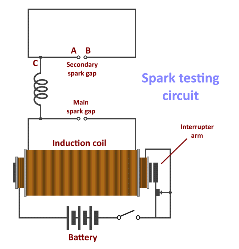
Hertz used a circuit similar to this to experiment with sparks
Hertz found that the only way to prevent sparks from being generated across the spark gap in the secondary circuit (Hertz called them "side sparks") was to connect the circuit so that connection point C was equidistant from points A and B. Hertz came to the conclusion that separate voltage waves must be traversing paths CA and CB. When both of these paths were the same length, then the voltages on each path would reach the gap in the secondary circuit at the same time, and would be in phase with one another. There would be no discernible voltage difference across the gap, and thus no spark; a spark will only be generated if there is a sufficiently large voltage difference between points A and B.
The electromagnetic waves reaching A and B are in phase. No spark is generated.
The electromagnetic waves reaching A and B are out of phase. A spark will be generated.
Hertz believed that the sparking at the main gap was producing electromagnetic waves. He likened the behaviour of the circuit to that of a tuning fork vibrating at its resonant frequency. The "vibrations" responsible for producing the electromagnetic waves were caused by the acceleration of electric charge within the circuit, and must be occurring at the circuit's natural, resonant frequency.
Hertz was aware from his studies that the resonant frequency of electrical vibrations in a circuit was dependent on the inductance and capacitance in the circuit. The phenomenon of electrical resonance had first been explored by French scientist Felix Savary (1797-1841) in 1826, and was subsequently the subject of further experimentation and theoretical treatments by a number of notable scientists, including American scientist Joseph Henry (1797-1878), British scientist William Thompson (1824-1907), and of course James Clerk Maxwell.
Hertz therefore continued his experiments, varying the inductance and capacitance in his test circuits. Hertz discovered that the length of the sparks produced by his spark gap circuits varied with frequency, and estimated that the resonant frequencies of his experimental circuits - known as LC resonator circuits because of they included both an inductive component and a capacitive component - must be in the order of tens of millions of cycles per second.
Hertz decided that the next step was to decouple the "side-spark" circuit from the main spark circuit. If Maxwell's theories of electromagnetic radiation were correct, the main circuit should radiate electromagnetic waves, which should carry electromagnetic energy to the nearby (but now separate) "side-spark" circuit, causing the charged particles within it to oscillate. In 1886, Hertz built his now famous "spark-gap transmitter", which is illustrated below.
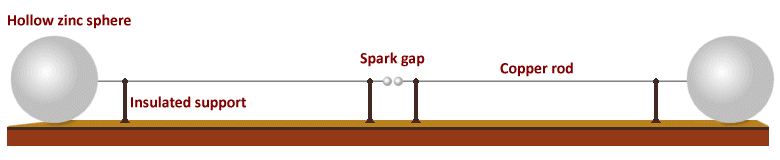
Hertz's "spark-gap transmitter"
Two hollow zinc spheres, each thirty centimetres in diameter, act as capacitors. A thin, one-metre long copper rod extends from each sphere to a point mid-way between the two spheres. The two equal-length rods are supported by four insulating posts made from sealing wax, and each rod is terminated by a small metal ball. There is an air gap of approximately 7.5 mm between the two terminating balls. An induction coil (not shown) is used to supply the high voltage alternating current needed to produce sparks across the spark gap.
Hertz's "receiver" was a copper wire rectangle approximately 120 × 80 centimetres, which had its own spark gap. When 20,000 volt pulses from the induction coil were applied to the apparatus, it behaved in the way Maxwell had predicted, producing electromagnetic waves at a frequency of about 50 MHz which Hertz was able to detect with his copper wire receiver, approximately a metre and a half from the transmitter, evidenced by tiny sparks occurring the receiver's spark gap.
Hertz had succeeded in generating and detecting radio waves - something Maxwell had only theorised, and a truly ground-breaking achievement. Hertz's own reaction to this breakthrough, however, indicates that he did not see it as having any particular application other than to prove the existence of a hitherto unseen natural phenomenon. In 1890, four years before his untimely death from a form of vasculitis at the age of thirty-six, he is reported to have said:
"I do not think that the wireless waves I have discovered will have any practical application."
The importance of Hertz's discovery may have been lost on Hertz himself, but others were quick to see its significance, among them the Italian inventor and electrical engineer Guglielmo Giovanni Maria Marconi (1874-1937). In 1897, Marconi founded the Wireless Telegraph & Signal Company, later to become the Marconi Company. In 1901 Marconi, in St. John's, Newfoundland, received the first ever transatlantic wireless transmission, sent from the company's high-power transmitting facility at Poldhu Point in Cornwall.
Frequency
In order to build efficient telecommunications systems and end-user equipment, it is essential to understand the fundamental properties of electromagnetic waves. We'll start with frequency, since we've already mentioned it several times.
Frequency (symbol: ƒ) is the term used to describe the number of oscillations (cycles) per second of a wave. The unit of frequency is the hertz (Hz), and one hertz is equal to one cycle per second. The term is named after the German physicist Heinrich Rudolph Hertz, who first produced and observed electromagnetic waves in 1887 (see above). The term is combined with metric prefixes to denote multiple units such as the kilohertz (10 3 Hz), megahertz (10 6 Hz), and gigahertz (10 9 Hz).
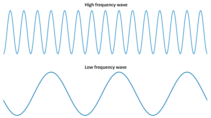
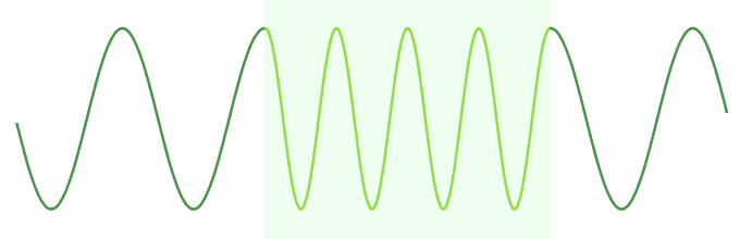
High frequency and low frequency waves
In telecommunications, a signal is composed of electromagnetic waves at various frequencies. Analogue telephone lines, for example, carry voice signals that occupy a frequency range of between 300 Hz and 3.4 KHz. We can measure the frequencies in a signal using an instrument called a spectrum analyser. In simple terms, the spectrum analyser takes an electrical signal as its input, and measures the amplitude of the signal across the range of frequencies that make up that signal. On the spectrum analyser's display screen, frequency is shown on the horizontal axis and amplitude is shown on the vertical axis.
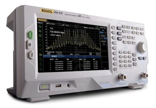
A Rigol DSA815-TG Spectrum Analyser
The spectrum analyser allows the user to observe and evaluate the spectral components of a signal, including the dominant frequencies, signal power, bandwidth, and distortion. It is frequently used in telecommunications to determine bandwidth usage, and to track down sources of interference. It can also be used to check the output of a wireless transmitter to ensure that the signals it transmits are within defined parameters for the type of equipment and intended use.
Amplitude
The amplitude of a wave is the maximum displacement from its rest position. You can think of it as being the maximum perpendicular distance between the wave and the axis about which it oscillates, or as the shortest distance between that axis and a peak or trough in the wave. For an electromagnetic wave, amplitude is directly related to the electromagnetic energy it carries.
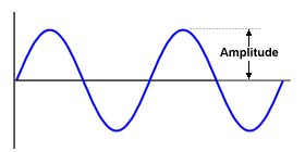
Amplitude is the maximum displacement from the rest position
Remember that electromagnetic waves are created by an electric field and a magnetic field oscillating in phase with one another. The amplitude of an electromagnetic wave can therefore be represented by the maximum field strengths of either the electric field or the magnetic field. The amplitude of the electric field is usually represented by the letter E, while the amplitude of a magnetic field is represented by the letter B.
The energy carried by an electromagnetic wave is proportional to its amplitude squared
The energy carried by a wave is proportional to its amplitude squared (this is true for all waves), so both the energy carried by an electromagnetic wave and its intensity I are proportional to the maximum field strength of both the electric field and the magnetic field. The intensity of an electromagnetic wave is the power of an electric or magnetic field per unit area, usually expressed in watts per square metre (W/m 2). For a continuous sinusoidal wave, the average intensity (I average ) is given by:
| I average = - | cε 0 E 02 |
| 2 |
where c is the speed of light, ε 0 is the permittivity of free space, and E 0 is the maximum electric field strength.
The average intensity can also be expressed in terms of magnetic field strength:
| I average = - | cB 02 |
| 2µ 0 |
where μ 0 is the permeability of free space, and B 0 is the maximum magnetic field strength.
We can also express the average intensity of an electromagnetic wave in terms of both electric field strength and magnetic field strength, since E 0 = c∙B 0 , as follows:
| I average = - | E 0 B 0 |
| 2µ 0 |
Wavelength
The wavelength (symbol: λ) of a wave is the distance between consecutive peaks (or consecutive troughs), measured in metres.
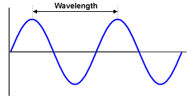
Wavelength is the distance between consecutive peaks
The discussion of wavelength here will concentrate on the wavelength of sinusoidal periodic waves, although the term wavelength can also be applied to non-sinusoidal periodic waves, and to the sinusoidal envelopes of amplitude-modulated waves. Note that in linear media any wave pattern can be described in terms of the independent propagation of sinusoidal components; non sinusoidal periodic waves are formed from the sum of a number of sinusoidal waves at different frequencies and amplitudes. As we saw above, the symbol normally used for wavelength is the lower case Greek letter lambda (λ).
The wavelength of an electromagnetic wave will depend on what type of electromagnetic wave we are dealing with. Gamma rays with a frequency of three hundred exahertz (300 × 10 18 Hz), for example, have a wavelength of one picometre (1 × 10- 12 m). At the other end of the electromagnetic spectrum, extremely low frequency (ELF) radio waves with a frequency of three hertz (3 Hz) have a wavelength of one hundred thousand kilometres (100,000 km) – nearly eight times the diameter of the Earth!
Note that the figures quoted above are for electromagnetic waves travelling in a vacuum at the speed of light, which is approximately three hundred million metres per second (3.0 × 10 8 m/s). EM waves travelling through a physical medium such as Earth's atmosphere will travel more slowly than they do in a vacuum, which means that waves with the same frequency will have a shorter wavelength when propagating through a medium than they will have when propagating through free space.
Wavelength decreases in a physical medium with slower propagation
For a sinusoidal waveform propagating at a fixed speed, whether through a medium or in free space, wavelength is inversely proportional to frequency. The relationship between wavelength, frequency and phase velocity (the speed at which the wave propagates through a medium) can be expressed as follows:
| λ = | v |
| f |
where λ is the wavelength in metres, v is the phase velocity in metres per second, and f is the frequency in hertz.
Two other properties of electromagnetic waves that you may encounter from time to time are the wavenumber (k) and the angular frequency (ω), both of which are directly related to wavelength and frequency.
The wavenumber of a wave (sometimes called the angular wavenumber) is the number of radians per unit distance (in contrast to frequency, which is the number of waves per unit time). The wavenumber can be expressed algebraically as follows:
| k = | 2π | = | 2πf | = | ω |
| λ | v | v |
The angular frequency of a wave, also known as radial frequency or circular frequency, measures angular displacement (the angle in radians through which a point rotates around a centre) per unit time, and has units of radians per second (rad s -1). The angular frequency can be expressed algebraically as:
| ω = 2πf = kv = | 2πv |
| λ |
Phase
In the context of electromagnetic waves, the term phase refers to a particular point in the cycle of a repeating waveform, measured as an angle in degrees or radians. One complete cycle of a periodic sinusoidal waveform occupies a phase space of three-hundred and sixty degrees (360°) or 2π radians (a phase space is a space in which all possible states of a system are represented, with each state corresponding to a single point in the phase space). The concept of phase is thus useful when we want to describe a specific point within a given cycle of a periodic wave. The diagram below illustrates the point.
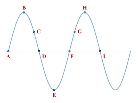
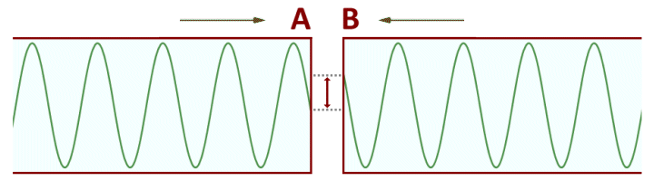
Two complete cycles of a periodic sinusoidal wave
In the above diagram, the first wave cycle starts at point A, which has a phase angle of 0 radians (0 degrees), and ends at point F, which has a phase angle of 2π radians (three hundred and sixty degrees). Note that, for the purposes of this article, we will use radians from now on when discussing phase angles. The wave reaches its positive peak at point B, which has a phase angle of π/2 radians. Points D and E have phase angles of π radians and 2π/3 radians respectively.
Points on consecutive waves that occupy the same unique position in the wave cycle have the same phase angle. Hence points B and H have the same phase angle, as do points D and I. Note, however, that two points on a sinusoidal waveform can have the same amplitude but different phase angles. Points A and D, for example, both lie on the horizontal axis that represents the waveform's rest position, but the wave is moving in different directions at these two points.
The same applies to points with the same amplitude on consecutive waves; points C and G both have the same amplitude, but point C lies within the second quadrant of the first complete cycle, where amplitude is decreasing, whereas point G lies within the first quadrant of the second cycle, where amplitude is increasing. The term quadrant here refers to a quarter cycle (π/2 radians).
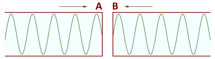
We are often interested in the phase difference between two waves, which can have various implications for signals used in telecommunications. Two sinusoidal waveforms of the same frequency are said to be in phase if they have the same phase angle at some arbitrary time t. Two sinusoidal waveforms of the same frequency that have different phase angles at time t are said to be out of phase. The following illustration shows two sine waves of the same frequency, but with a phase difference of π/2 (one quarter-cycle):
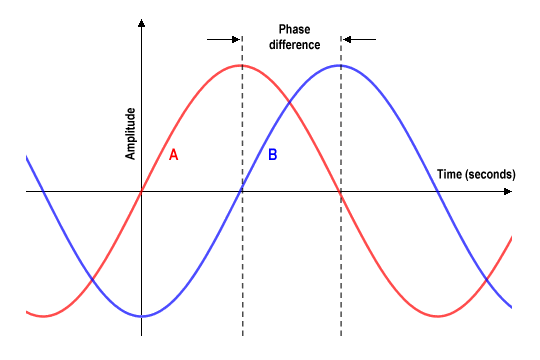
Two sine waves out of phase by π/2
By convention, the phase difference between two waves of the same frequency is expressed as a value in the range -π to +π. In other words, the first wave can lead the second wave by anything up to π radians. The second wave is said to lag the first wave. When two signals differ in phase by exactly -π/2 or +π/2 radians, they are said to be in phase quadrature. (in the illustration above, wave A leads wave B by π/2 radians). When two signals differ in phase by exactly π radians, they are said to be in phase opposition.
On a linear medium, two sinusoidal waves of the same frequency and amplitude that are in phase will add together to produce a wave with an amplitude that is equal to the sum of the amplitudes of the two waves:
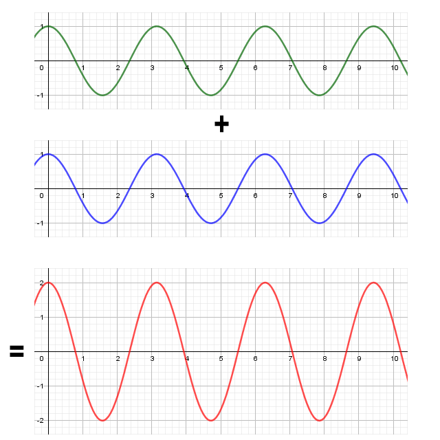
The sum of two waves with the same frequency and phase
Two sinusoidal waves of the same amplitude and frequency that are in phase opposition will also sum together, but this time the waves will effectively cancel each other out because the sum of the corresponding points on each wave is zero:
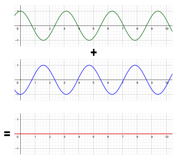
The sum of two waves with the same frequency but in phase opposition
If two sinusoidal waves with the same frequency but different amplitudes are in phase opposition, the result will be a sinusoidal wave of the same frequency, but with an amplitude equal to the difference in amplitudes of the original two waves, and with the same phase as the larger of the two original waves.
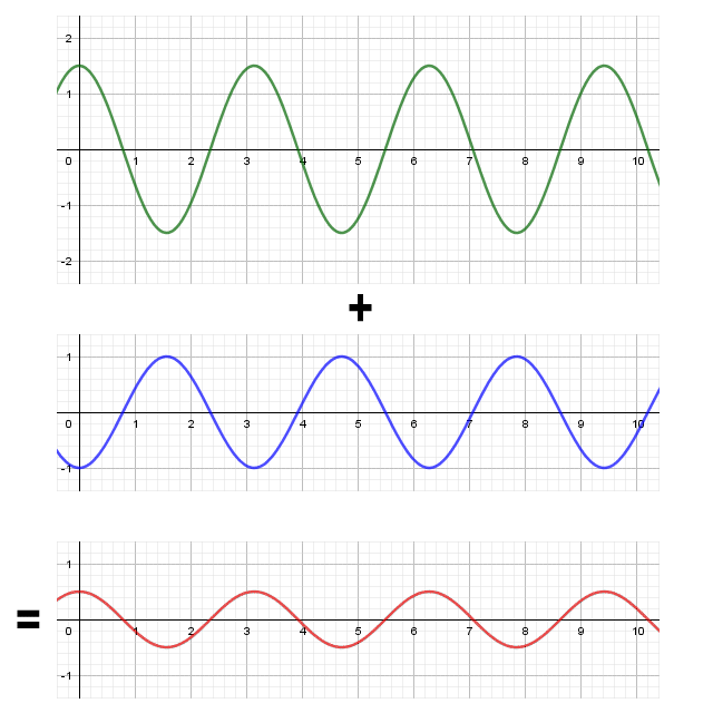
The sum of two waves with the same frequency but different amplitudes, in phase opposition
The phase difference between two waves of the same frequency moving past a fixed point is a function of the time difference between the same positions within the wave cycles, usually expressed as an angle in radians. The phase angle φ of a point on a wave passing a given point at time t is expressed as φ(t). For a sinusoidal wave, the value of φ(t) for a given value of t is given as:
| φ(t) = 2π ⟦ | t - t0 | ⟧ |
| T |
where:
t0 is an arbitrary time value chosen as the start of the wave cycle,
T is the period of the wave (i.e. the inverse of the frequency, or f -1), and
⟦...⟧ is mathematical notation that denotes the fractional part of a real number.
Note that the two points being compared may be several wave cycles apart. This would result in a fractional value that includes an integer component when we divide the time difference between the two points by the period of the wave, because it will include some whole number of cycles. The double square bracket notation ⟦...⟧ is used to indicate that the integer part of the result should be discarded. Note also that t 0 is usually chosen to be any value of t at which the amplitude of the wave changes from zero to a positive value.
The phase difference between two sinusoidal waves becomes particularly significant for waves propagating through a linear transmission medium, because the waveforms will add together to create a new waveform. We have already seen the result of adding sinusoidal waves of the same frequency together, both when they are in phase, and when they are in phase opposition. Clearly, the result of adding two waves together is going to depend on the phase difference between them.
The interaction of different waves on the same medium is called interference. If the phase difference between two waves of the same frequency is zero, the signals will reinforce each other (this is called constructive interference). When the waves are in phase opposition the interaction between them is called destructive interference. For any other scenario in which there is a phase difference between two waves of the same frequency, the resulting wave will depend on the actual phase difference and the respective amplitudes of the two waves.
The question of phase is of interest to telecommunications engineers and the designers of telecommunications systems for a number of reasons. Changes in phase can be used, for example, to modulate a carrier wave, enabling digital information to be encoded into a signal (a modulation technique known as phase shift keying).
Phase difference is also a potential cause of interference in unguided media. Radio signals, for example may follow different paths from the transmitter to the receiver, as is the case when one signal travels directly to the receiver from the transmitter, and a copy of the signal is received as the result of the signal being reflected by a nearby building. The reflected signal will have followed a longer propagation path, and will thus lag the direct signal slightly.
Phase velocity
The phase velocity (or phase speed or wave speed) of an electromagnetic wave is the speed at which a phase of a wave is propagated through a medium. All electromagnetic waves travel at the speed of light, c (circa three hundred million kilometres per second), through the vacuum of space, but the speed at which a wave propagates through a physical medium will depend on the properties of the physical medium and the wavelength of the wave.
The phase velocity of a wave v p is related to the wavelength λ and the period T of the wave, as follows:
| v p = | λ |
| T |
We can also express phase velocity as the product of wavelength λ and frequency f:
v p = λ f
Phase velocity can also be expressed in terms of the wave's angular frequency ω and its wavenumber k (see above) as follows:
| v p = | ω |
| k |
We have stated that the speed at which am electromagnetic wave travels through a physical medium will be slower than the speed at which it propagates through free space (i.e. the speed of light in a vacuum, or circa 300 million metres per second). The speed of propagation through a particular medium will depend on three factor: the linearity of the medium, the frequency of the wave, and the refractive index of the medium.
We'll deal with linearity first. For the purposes of this article, we use the term linear medium to indicate that electromagnetic waves can propagate through the medium without distortion. There is a more formal definition, which states that a linear medium is one that allows superposition. This is essentially what happens when two or more waves of the same type are travelling on the same medium; the amplitude of the resulting waveform at any point is equal to the sum of the displacements at that point due to each individual wave.
The frequency of a wave will not change when the wave enters some physical medium, but its wavelength will get shorter because the wave has slowed down. Why? To answer that question, we have to delve into the realm of quantum mechanics, but we'll try to keep it as simple as possible.
Essentially, when an electromagnetic wave encounters the atoms in the physical transmission medium, its energy is absorbed. This causes the electrons within the atoms to vibrate for a short interval of time, after which the vibrating electrons create a new electromagnetic wave with the same frequency as the original electromagnetic wave.
When the energy of an electromagnetic wave is re-emitted by an atom, it travels through the space between atoms until it encounters the next atom, where the process of absorption and re-emission is repeated. The period of time during which the electrons are vibrating is incredibly short, but it nevertheless slows down the propagation of the wave through the medium.
The degree to which a physical medium will affect the phase velocity of an electromagnetic wave is determined by the medium's refractive index, n. This can be expressed as follows:
| v p = | c |
| n |
where v p is the phase velocity, c is the speed of light, and n is the refractive index of the medium. The refractive index of a material also varies with wavelength. Evidence of this can be seen when white light passes through a prism and is split into its constituent colours. For most media, refractive index tends to increase with frequency. For example, within the visible light spectrum, refractive index is higher for blue light than for red light.

Refractive index is higher for blue light than for red light
Note that for transmission media involving conducting materials such as copper wire, the phase velocity is more often defined using a property of the conducting material called the dielectric constant. Without going into a detailed explanation here, it can be shown that the dielectric constant k is equal to the square of the refractive index n, i.e. k = n 2. We can thus express the phase velocity v p of an electromagnetic wave in a linear conducting medium as:
| v p = | c |
| √k |