| Author: | |
| Website: | |
| Page title: | |
| URL: | |
| Published: | |
| Last revised: | |
| Accessed: |
Let's suppose we have some non-linear function ƒ(x). If we draw the graph of the function, it will give us a curve. The tangent to the curve, at some point on the curve, is the straight line that touches the curve at that point but (in most cases) does not cross it (we will talk about the exception in due course). The slope of the tangent to a curve at a point is also the slope of the curve itself at that point. As you should by now also be aware, the slope of a function at a specific point gives us the instantaneous rate of change (otherwise known as the derivative) of the function at that point. If we want to know the slope of a function for a given value of x, we simply need to obtain the derivative function (by applying the appropriate rules of differentiation), and then apply the derivative function to that value of x to get the slope. Here is the graph of the function ƒ(x) = x 3 + 2x + 4:
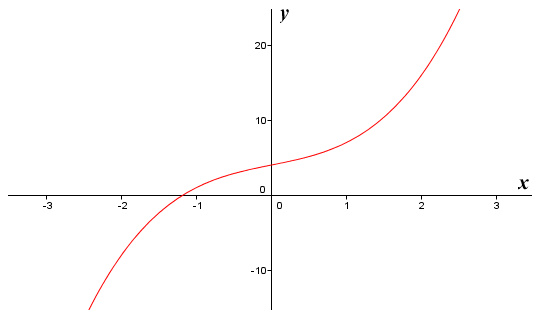
The graph of the function ƒ(x) = x 3 + 2x + 4
Let's now suppose that we want to know the gradient of the function at x = 1. We can find the derivative function by applying the basic rules of differentiation:
ƒ′(x) = 3x 2 + 2
If we now apply ƒ′(x) to x = 1 we get:
3x 2 + 2 = 3 × 1 + 2 = 5
The slope of the function at x = 1 is therefore five (5).
The slope of the tangent to some point on a curve (called the point of tangency) is the same as the slope of the function that produces the curve at that point. Points on the curve that are close to the point of tangency will also be close to the tangent line. This means that, close to the point of tangency, the linear function that produces the tangent line as its graph will be a reasonably accurate approximation of the non-linear function that produces the curve itself. Thus, we can approximate a non-linear function locally using a linear function. We call this a linear approximation (you might also come across the terms straight line approximation and tangent line approximation, which mean the same thing).
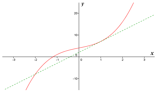
A tangent to a non-linear curve has the same slope as the curve at the point of tangency
We have seen that we can find the slope of the tangent to a function ƒ(x) easily enough by finding the derivative function ƒ′(x) and applying it to the x value corresponding to the point of tangency. What we want, however, is to derive the linear function that produces the tangent line (and hence the function that gives us the linear approximation of ƒ(x) near the point of tangency). We can do this using the information we have to hand. Consider first of all the formula for finding the slope of a straight line. You may recall that if we have two points with xy coordinates x1, y1 and x2, y2, the general formula for finding the slope m of the straight line that intersects both points is:
| m = | y2 - y1 |
| x2 - x1 |
where m is the slope of the line and x1, y1 and x2, y2 are the x and y coordinates of any two points on the line. Now consider the information available to us. We have the x coordinate of the point of tangency (because we chose it). We can find the y coordinate of the point of tangency simply by applying ƒ(x) to its x coordinate. We will assign the values of the x and y coordinates of the point of tangency to the variables x1 and y1 in our formula respectively. We can now obtain the slope m of the tangent line by applying the derivative function ƒ′(x) to x1. Now we just need to modify the formula for finding the slope of a straight line somewhat to suit our purposes as follows:
| m = | y - y1 |
| x - x1 |
We can rearrange this to get the point-slope form of the formula:
y - y1 = m (x - x1)
We can rearrange once more to leave y alone on the left hand side of the equation:
y = m (x - x1) + y1
Let's apply this to the function ƒ(x) = x 3 + 2x + 4 which we saw above to derive the linearisation of ƒ(x) at x = 1, which we will call L(x). First of all we'll find the value of y1:
y1 = x 3 + 2x + 4 = 1 + 2 + 4 = 7
Now we will find the slope m of the function:
m = 3x 2 + 2 = 3 + 2 = 5
Substituting these values into our revised equation we get:
y = m (x - x1) + y1 = 5x - 5 + 7 = 5x + 2
Thus:
L(x) = 5x + 2
Here once more is the graph of the non-linear function ƒ(x) = x3 + 2x + 4, together with the graph of its linearisation L(x) = 5x + 2, which gives us the tangent to the curve at x = 1.
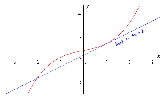
The graphs of the functions ƒ(x) = x3 + 2x + 4 and L(x) = 5x + 2
Let's suppose we want to find the approximate value of a function ƒ(x) for values of x near to x = c. We can rewrite our formula for the linearisation (i.e. the tangent line to the graph of ƒ(x) at x = c) purely in terms of the function ƒ(x), and its derivative ƒ′(x), as follows:
ƒ(x) ≈ ƒ′(c) (x - c) + ƒ(c)
For values of x that are sufficiently close to c, this will give us a reasonably accurate approximation, because as you may remember, the closer we zoom in on a curve at a point, the more the curve resembles the tangent line at that point. If ƒ(x) is concave down in the interval between x and c, the approximation will be higher than the actual value of ƒ(x). If ƒ(x) is concave up in the interval between x and c, the approximation will be lower than the actual value of ƒ(x). We can illustrate this point quite nicely using a cubic function, since all cubic functions have an inflection point (i.e. a point where the function changes concavity). Here is the graph of the cubic function ƒ(x) = x 3 - 4x + 10, together with the graph of its linearisation L(x) = -4x + 10, which gives us the tangent to the curve at x = 0.
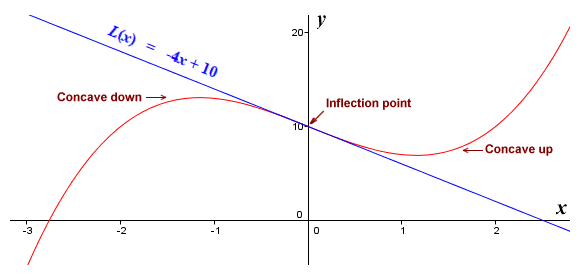
The graph of the functions ƒ(x) = x 3 - 4x + 10 and L(x) = -4x + 10
We mentioned earlier that the tangent to a curve touches the curve at a single point, but does not usually cross the curve at that point. The exception occurs when the point of tangency coincides with an inflection point (a point where the curve changes concavity), as it does here. You can clearly see from the illustration that the approximation given by L(x) will give a lower value than ƒ(x) for values of x that are greater than zero (where the function curve is concave up) and a higher value than ƒ(x) for values of x that are less than zero (where the function curve is concave down). Fairly obviously, the further away we get from x = c, the less accurate the approximation becomes.
The range of x values over which we get an acceptable approximation will depend on a number of factors. For example, it depends on the type of function being used, the point of tangency chosen, and the degree of accuracy actually required. Linear approximation can be useful on occasion because they allow us to simplify formulas and still achieve reasonably accurate results. They can allow us to make rough estimates in order to make sure we are on the right track with more complex calculations. When modelling complex systems, scientists and engineers can use them to quickly make reasonably accurate predictions about the behaviour of parts of the system without having to wait for large-scale computer simulations to reach completion.
In addition to finding the formula that gives us the tangent to a curve at a given point, it is often desirable to be able to find the formula that gives us the normal to the curve at some point on the curve. The normal to a curve at a specified point is the line that is perpendicular (at right-angles) to the tangent to the curve at that point. The illustration below shows the graph of the function ƒ(x) = x 2, the tangent to the graph at x = 1, and the normal to the curve at x = 1. Note that the normal is perpendicular to both the tangent and the function curve itself at the point of tangency.
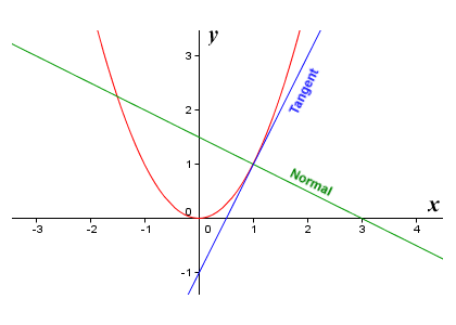
The graph of the function ƒ(x) = x 2, together with the tangent and the normal at x = 1
We have already seen how to derive the linear function that produces the tangent line to a curve at a specific point on the curve. We can derive the linear function that produces the normal using a similar method. We have the x coordinate of one point on the normal, because it passes through a point of tangency which we have chosen. As previously, we can find the y coordinate of the point of tangency by applying ƒ(x) to the x coordinate. We know that the slope m of the tangent is found by applying ƒ′(x) to the x coordinate of the point of tangency. We know that the normal is perpendicular to the tangent line. If two lines are perpendicular to one another, their slopes are opposite reciprocals of one another, and the product of their slopes is therefore always minus one (-1). This fact allows us to derive the following formula for the normal line:
| y = | -1 | (x - x1) + y1 |
| m |
Let's look at an example. The illustration below shows the graph of ƒ(x) = x 3 - 3x, together with the tangent line and the normal at x = 2. We will apply what we have discussed so far to derive the formulae for the tangent line and the normal.
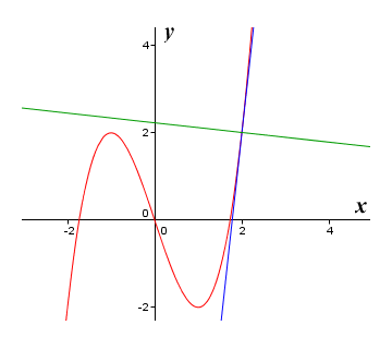
The graph of the function ƒ(x) = x 3 - 3x, together with the tangent line and the normal at x = 2
First we apply the rules of differentiation to find ƒ′(x):
ƒ′(x) = 3x 2 - 3
Next we will find the slope m of the tangent at x = 2:
m = 3x 2 - 3 = 3 × 4 - 3 = 9
Now we will find the y coordinate of the point of tangency (the formula variable y1):
y1 = x 3 - 3x = 8 - 6 = 2
We now have all the information we need in order to derive the linearisation of ƒ(x) at x = 2, which we will call L(x):
L(x) = m (x - x1) + y1 = 9x - 18 + 2 = 9x - 16
We can also derive the formula for the normal line:
| y = | -1 | (x - x1) + y1 = | -1 | (x - 2) + 2 |
| m | 9 |
| y = | -1 (x - 2) + 18 | = | 20 - x |
| 9 | 9 |
It is important to be able to calculate the normal to an arc or a curved surface in a number of applications. One such application is computer graphics, where the programmer must be able to determine the degree to which light from a known source is reflected from a point on a curved line or surface for the purpose of shading the pixel representing the point (i.e. determining the colour and intensity at which the pixel should be displayed). Another important application is found in optics, a branch of physics dealing with the behaviour of light. For example, when a ray of light travels from one transparent medium into another, the angle at which it is incident upon (i.e. meets) the boundary between the two materials, and the angle through which it is refracted (i.e. bent) as it passes through that boundary, are both measured with reference to the normal (the line at right angles to the curved line or surface at the point of entry).
Just as we re-wrote the formula for the tangent line to the graph of ƒ(x) at x = c in terms of the function ƒ(x) and its derivative ƒ′(x), we can also re-write the equation for the normal line to the graph of ƒ(x) at x = c as follows:
| y = | -1 | (x - c) + ƒ(c) |
| ƒ′(c) |